
Semiconductor Spin Qubits
Accelerate spin-qubit tune-up, control, and readout with synchronized DC, RF, microwave, and baseband orchestration. Unlock real-time workflows that take you from first electrons to scalable QPU operation.


Research
Semiconductor quantum dot spin qubits use single electrons or holes confined by electrostatic gates and cooled to cryogenic temperatures. Their spin state serves as the qubit, enabling robust quantum information encoding in a platform that is compatible with advanced silicon fabrication. With a nanometer scale footprint, spin qubits offer a highly scalable path toward practical quantum computing.
Operating spin qubits require precise control of both charge and spin. Electrostatic electrodes define the quantum dots and tune electron occupancy with single electron precision. A global magnetic field separates the spin states, while coherent control is achieved through carefully shaped RF, microwave, and baseband pulses.
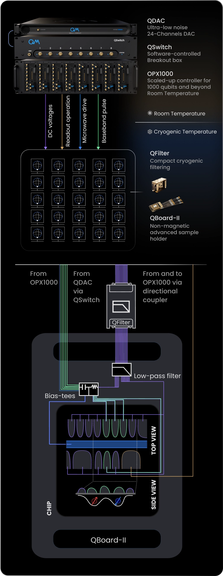
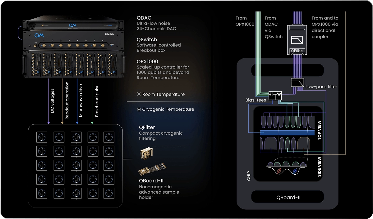
Quantum Machines’ Orchestration Platform supports the full spin qubit workflow. QPU tune up begins with accurate modulation of the confining potentials, enabled by the QDAC-II ultralow noise DC source and the QSwitch automated reconfiguration matrix. Once the potential landscape is established, single qubit gates can be driven using microwave transitions or baseband control. Coupling between spins is then controlled through fast, high fidelity baseband pulses that tune exchange interactions. The OPX1000 hybrid controller provides the pulse generation, timing precision, and real time orchestration required for these operations.
Together, Quantum Machines’ control stack delivers stable signals from room temperature to the cryogenic device, supports multidimensional optimization, and enables advanced real time workflows through QM’s Hybrid Control.
Set Up Architecture
Quantum-Classical Integration and Control Highlights
First electrons to full high‑fidelity characterization
The promise of spin qubit systems relies crucially on the ability to mitigate crosstalk in gates, drifting potentials, and low‑level waveforms that are difficult to stabilize. Quantum Machines’ Orchestration Platform shortens the entire path from first contact to randomized benchmarking with stable, calibrated, high-fidelity qubit operations.
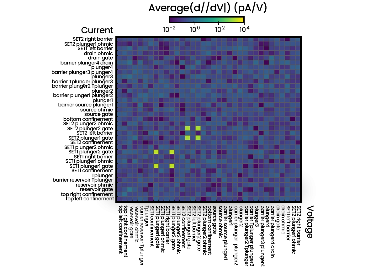
Whether the qubit encoding is Loss-DiVincenzo with synthetic spin–orbit fields, singlet-triplet qubits, or exchange‑only qubits, the combination of OPX1000 pulse control and QDAC-II ultralow noise DC delivery enables fully synchronized gate operations, readout, and analog feedback from a single deterministic timing engine. Early characterization steps such as leakage‑matrix measurements, stability‑diagram acquisition, and identification of single‑electron regimes are dramatically accelerated, with QDAC‑II’s native current measurements.
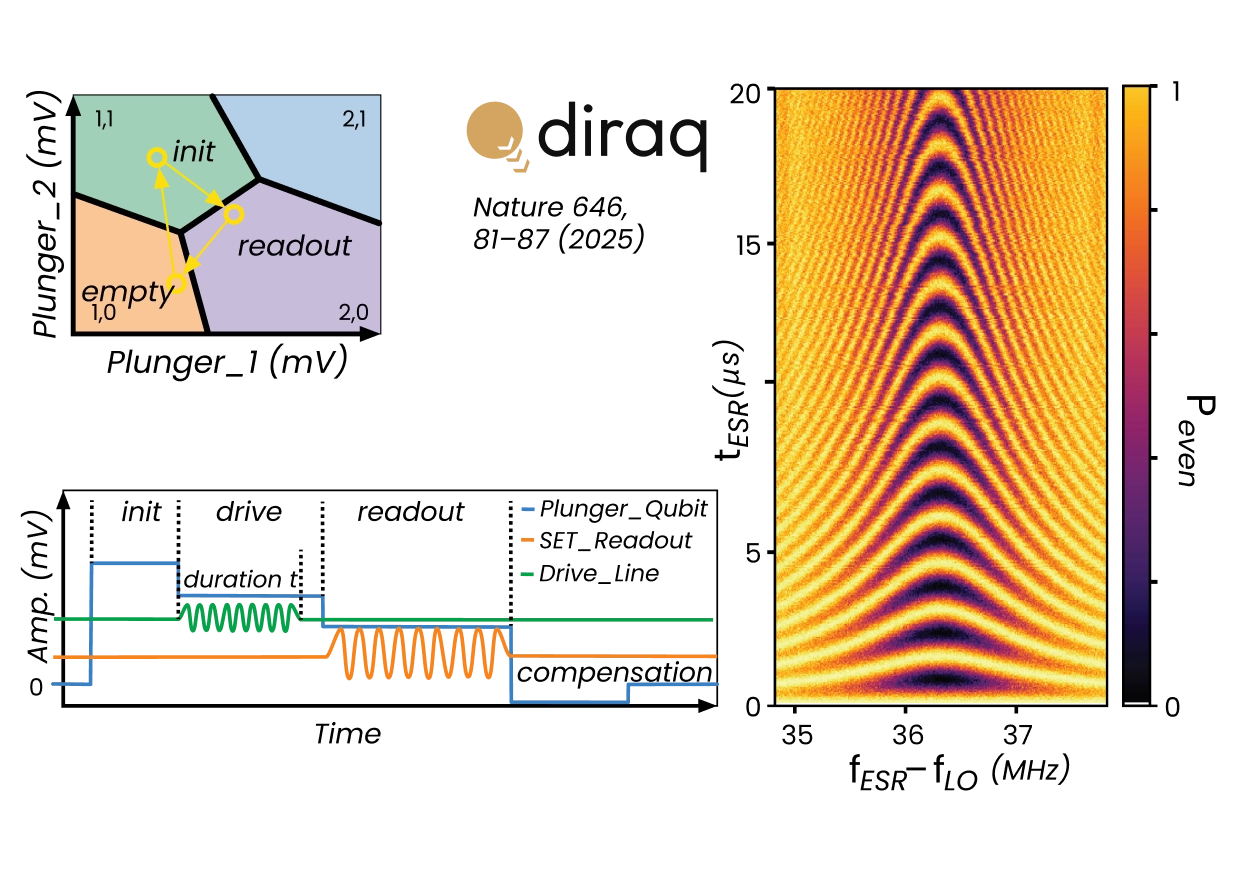
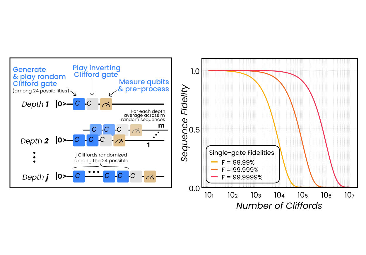
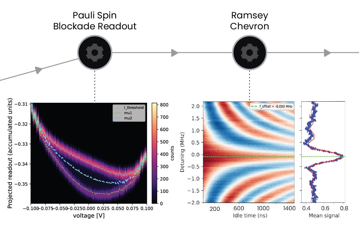
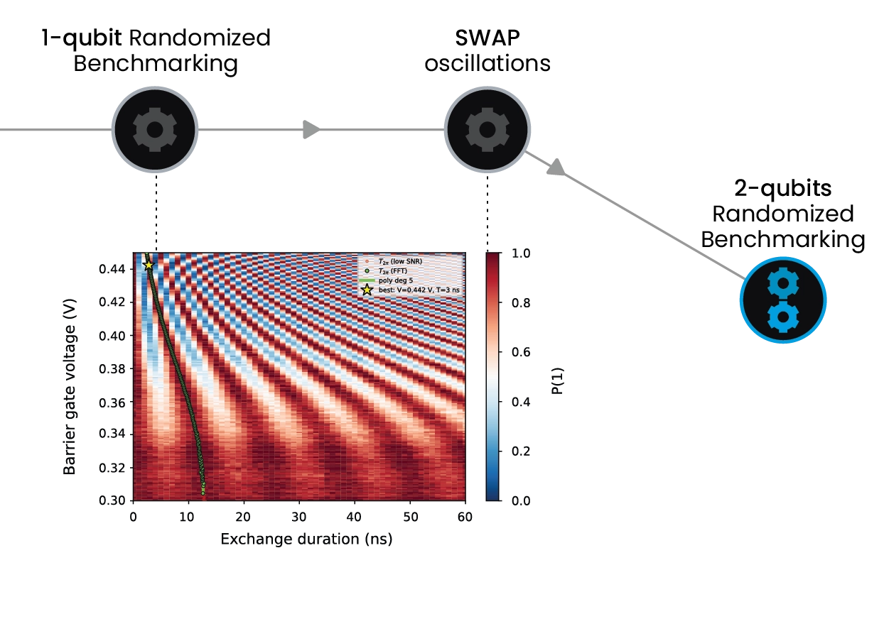
Once the device is operating in its qubit regime, the hardware natively supports both Pauli spin blockade and Elzerman readout, with all sequencing, alignment, timing waits, and data acquisition executed inside QM’s unique Pulse Processing Unit. OPX instructions are evaluated in real time allowing long duration experiments such as seconds‑long T₁ measurements with limited overhead, and reducing drift susceptibility. For coherent control, the OPX1000 generates high-purity ESR tones, shaped exchange pulses, and dynamically varying detuning ramps, making multi-parameter spectroscopy, Rabi, and 2D Chevron scans easy and fast. Entire maps can be captured before averaging, significantly suppressing slow environmental drift and improving extraction of resonance and coherence parameters. OPX1000 and the intuitive QUA language allow for randomized‑benchmarking sequences, going from system, bringing up to qubit control and fidelity optimization to be performed in a matter of 48 hours.
Video mode for rapid, modular and user-friendly spin qubit tune-up
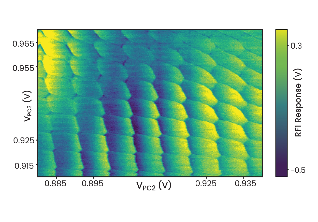
Tuning up quantum dots is a multi-dimensional parameter space optimization process. Quantum Machines’ solution speeds up tuning spin qubits using video mode. By relying fast readout, with bandwidth ranging from MHz to GHz, charge stability diagrams can be streamed from the OPX to the client PC reaching a refresh rate up to 20 fps. Thanks to three tightly coupled modules, a data acquirer, a scan mode, and an inner loop action, implemented using QUA, video mode allows for a truly interactive tune-up experience.
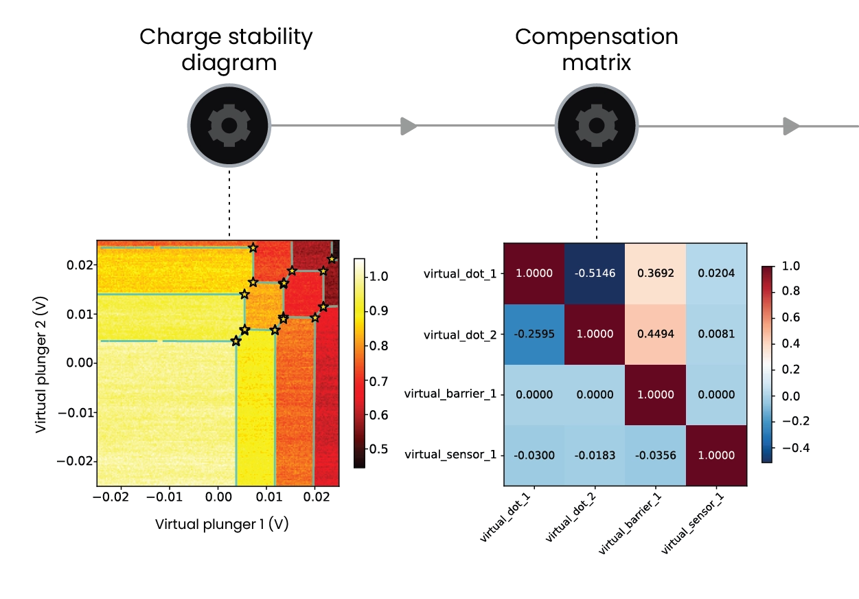
Using the ScanModes() abstraction, video mode defines how 2D charge stability diagrams are sampled in a virtualgate parameter space. The InnerLoopAction() specifies the operation executed at each sampled point after setting the scan parameters. The VideoMode() class manages streaming to the frontend, where data are visualized through a webbased interface that allows scan parameters to be dynamically modified. Integrated virtual gate layers support dottodot and sensor compensation, allowing realtime updates of virtual gate matrices and DC biasing directly from the GUI, with immediate feedback in the charge stability diagram.

From Qubits to QPU, with QUA-enabled real-time control
QUA, QM’s pulse-processing language, enables deterministic DC control, fast pulse sequencing, and realtime readout within a single program, without repeated client–hardware interaction in spin qubit experiments. For example, chargestabilitydiagram acquisition can be implemented by coordinating QDACII voltage stepping with OPX1000 generated trigger pulses and reflectometry readout. Nested loops in QUA define the scan geometry, while functions such as play(), wait(), and measure() synchronize voltage updates and data acquisition.
Constructs such as loops, conditionals, arithmetic operations, and switch statements allow experiments to branch dynamically based on program variables or measurement outcomes. QUA and OPX1000 allow for closedloop routines such as PID stabilization of chargesensor, simplify the construction of complex voltagepulse sequences, and enable highlevel abstractions such as the VoltageGateSequence() class to define pulse trajectories directly in gatevoltage space. Builtin compensation ensures zero net DC offset, while dynamic crosstalk correction can be applied through configurationlevel crosstalk matrices, mitigating unintended perturbations of neighboring qubits in dense arrays.
Ultimately, by embedding sequencing, feedback, and data handling directly into the execution layer, QUA reduces experimental overhead and allows the user to focus on physics rather than control.


“Dedicated hardware for controlling and operating quantum bits is something we have all been dreaming of. Quantum Machines has answered this call by allowing us and others in the field to scale up with ease and with far greater functionality than was ever possible before. “

Prof. Amir Yacoby
Professor
“OPX has been a powerful enabler in our lab, helping us quickly characterize the performance of our recently discovered qubits. The hardware removes time wasted in uploading and waiting during pulse programming. QUA has substantially reduced the complexity of writing quantum protocols, allowing us to code dynamical decoupling and RB sequences in just a few lines. It remarkably saves our time in optimizing the processes and visualizing the results, allowing us to focus more on understanding the physics of our new qubits.”

Prof. Dafei Jin
Professor
"OPX+ & Octave: Perfect, all-in-one measurement system for SNU's silicon 5 qubit device!"

Prof. Dohun Kim
Professor
“The OPX’s fast feedback and unique real-time processing capabilities were critical for our experiment. Combining these with the OPX’s intuitive programming and QM’s state-of-the-art cryogenic electronics allowed us to do something that we have dreamt of doing for years.”

Prof. Ferdinand Kuemmeth
Professor

Blog
Blog
Quantum Machines’ Latest Acquisition Highlights Europe’s Growing Quantum Talent Base
Read more June 2026 | 4 min read
Scientific Publications
Loss Mechanisms in High-coherence Multimode Mechanical Resonators Coupled to Superconducting Circuits
Read more May 2026 | 1 min read
Scientific Publications
Learning Nonlinear Heterogeneity in Physical Kolmogorov-Arnold Networks
Read more May 2026 | 1 min readFAQs
How fast can a system go from first electrons to high-fidelity characterization?
The platform is built to shorten the entire path from first contact to randomized benchmarking with stable, calibrated operations. Early steps like leakage-matrix measurements, stability-diagram acquisition, and identifying single-electron regimes are accelerated using QDAC-II’s native current measurements. In practice, the combination of OPX1000 and QUA enables going from system bring-up to qubit control and fidelity optimization in a matter of 48 hours.
What spin-qubit readout methods does the platform support?
The hardware natively supports both Pauli spin blockade and Elzerman readout, with all sequencing, alignment, timing waits, and data acquisition executed inside the PPU. Because OPX instructions are evaluated in real time, long-duration experiments such as seconds-long T₁ measurements run with limited overhead and reduced drift susceptibility. For coherent control it generates high-purity ESR tones, shaped exchange pulses, and dynamic detuning ramps for Rabi and 2D Chevron scans.
What is video mode, and how does it speed up tune-up?
Video mode makes the multidimensional tune-up of quantum dots interactive by streaming charge-stability diagrams from the OPX to the client PC at refresh rates up to 20 fps, using fast readout with bandwidth from MHz to GHz. It’s built from three tightly coupled QUA components: a data acquirer (ScanModes()), an inner-loop action (InnerLoopAction()), and streaming management (VideoMode()). Integrated virtual-gate layers let you update virtual-gate matrices and DC biasing directly from the GUI, with immediate feedback in the diagram.
How does QUA enable real-time spin-qubit control?
QUA enables deterministic DC control, fast pulse sequencing, and real-time readout within a single program, without repeated client–hardware interaction. Constructs like loops, conditionals, arithmetic, and switch statements let experiments branch on measurement outcomes, and abstractions such as VoltageGateSequence() define pulse trajectories directly in gate-voltage space. Built-in compensation maintains zero net DC offset while configuration-level crosstalk matrices mitigate perturbations of neighboring qubits in dense arrays.

Scale
Semiconductor spin qubits offer a highly scalable path to quantum computing, but moving from individual qubits to large QPUs requires more than precise control. It demands an orchestration layer that can handle dense device layouts, parameter drift, signal distortions, and increasingly complex calibration workflows.
Quantum Machines’ Orchestration Platform provides the control architecture needed to scale spin-qubit systems. With OPX1000 at its core, it enables synchronized pulse generation, real-time processing, and deterministic control across growing qubit arrays. Digital filtering helps preserve signal fidelity at the device, compensating for distortions across complex signal paths.
Scaling also requires automation and higher levels of software abstraction. QM’s QuAM architecture provides an object-based representation of the QPU, allowing quantum operations to be parameterized at the qubit level and significantly reducing programming complexity for large-scale processors. Standardized QuAM sequences can be combined within QUAlibrate routines to build complex calibration graphs that support tune up automation and parallel execution. Together with QM’s Open Acceleration Stack, these tools integrate advanced optimization and machine-learning workflows directly into the calibration loop, enabling fast tune-up, drift correction, and scalable operation of spin-based quantum processors.
Set Up Architecture


Quantum-Classical Integration and Control Highlights
Firmware for large scale spin qubit QPU control
The OPX firmware provides the signal-integrity backbone required for low-noise, stable, distortion-free spin qubit control across complex pulse sequences.
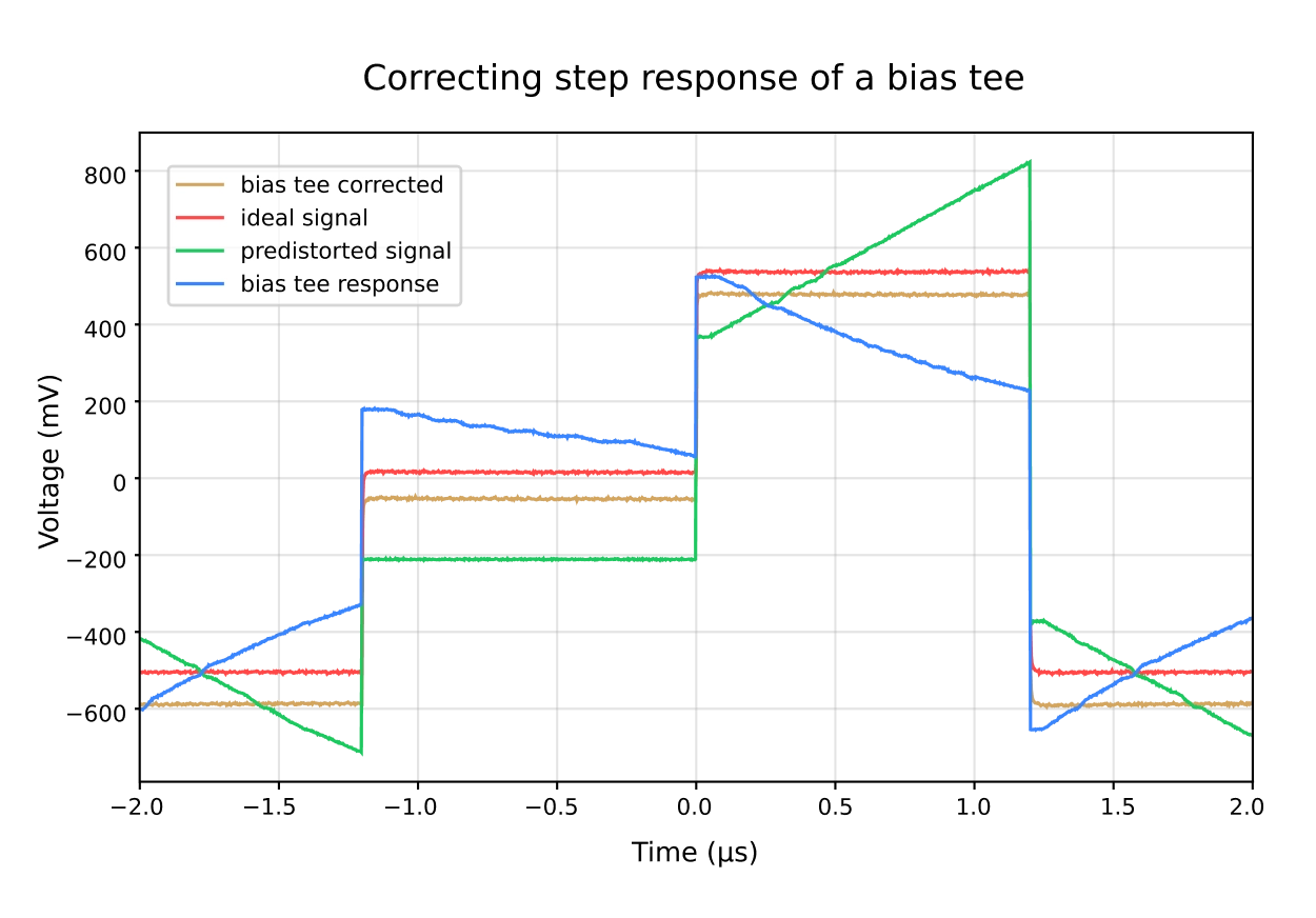
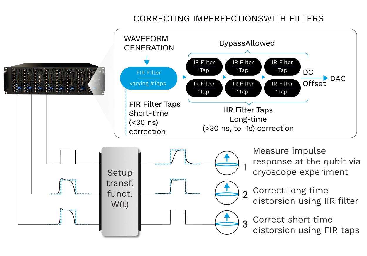
Digital filtering is implemented directly in firmware, with native FIR and IIR filters available for any pulse element. IIR filters compensate distortions from bias-tees, while FIR filters support sub-nanosecond baseband rise times and skew control at picosecond-level resolution. Because filtering runs on the Pulse Processing Unit, pulse predistortion is applied in real time, reducing memory use and minimizing experiment run time.
The firmware also manages line-shape correction and synchronized timing across DC, RF, and readout channels. Crosstalk compensation matrices can be embedded in the configuration file, enabling real-time correction of capacitive coupling between adjacent gates. For rapid, multidimensional voltage sequences, the system can automatically generate compensation pulses to maintain zero net DC offset.
The same real-time engine further supports stabilization routines such as onboard PID loops for drift-sensitive charge sensors, with update rates of a few hundred nanoseconds. Error signals, thresholds, and correction voltages are computed in firmware, allowing experiments to adapt continuously to quasi-static charge rearrangements without interruption.
Abstraction and Automated Calibrations with QM’s Orchestration
Tune-up and characterization are only the beginning of operating spin-qubit systems. Over time, charge environments shift, gate voltages drift, tunnel couplings change, and optimal operating points move. QM’s Orchestration Platform is designed to make both bring-up and retuning of spin-qubit systems fast, automated, and scalable processes.
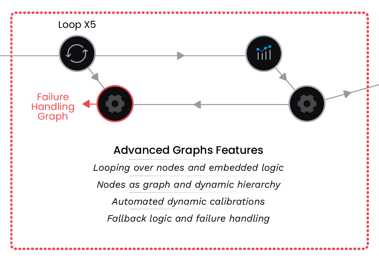
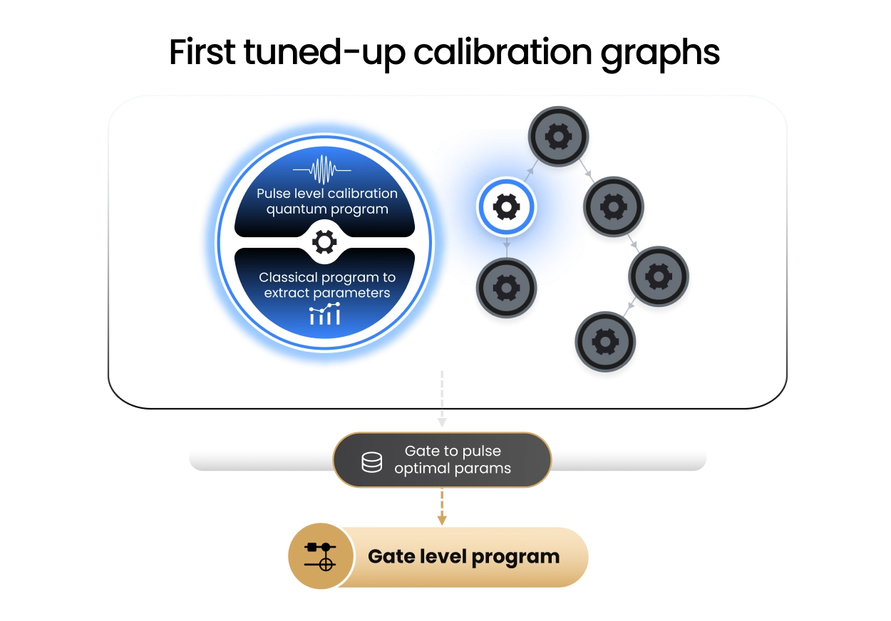
QUAlibrate transforms QUA protocols and tuning routines into nodes of a calibration graph. In spin-qubit platforms, these nodes can include gate virtualization, Loss-DiVincenzo-style calibration routines, charge-stability scans, sensor optimization, dot tuning, tunnel-rate calibration, Pauli spin blockade readout optimization, exchange calibration, and single- and two-qubit gate tune-up. These routines can be automated, enriched with decision logic, and parallelized across many dots and qubits.
QUAlibrate is built around QuAM, which provides the structured device model used across calibration nodes. For spin qubits, QuAM enables users to define their spin qubit abstraction based on the target QPU architecture, including Loss-DiVincenzo, exchange-only, or singlet-triplet implementations. It also incorporates shuttling architectures, enabling streamlined tune-up and deployment of large multi-core spin-qubit QPUs.
This makes calibration routines hardware-aware, reusable, and scalable. Together with real-time PPU compute and QM’s Open Acceleration Stack, QUAlibrate and QUAM help automate retuning, handle drift, and accelerate the path from device bring-up to reliable spin-qubit control.
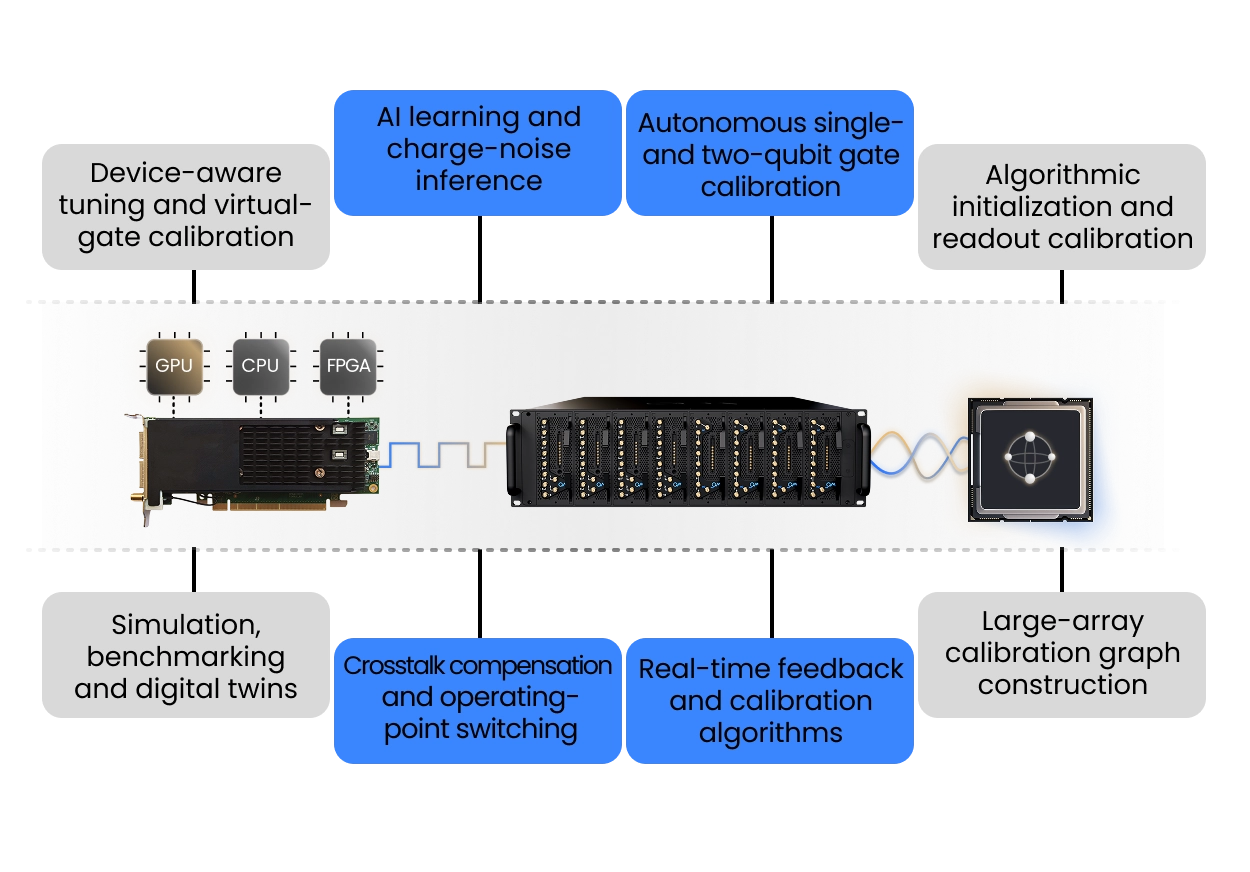
Real-time embedded calibrations with QM’s Open Acceleration
Large scale quantum processors require calibrations that run continuously, adaptively, and without interrupting quantum programs. QM’s Open Acceleration Stack connects the OPX1000 to external CPUs, GPUs, and FPGAs through low-latency links, allowing calibration routines to be embedded directly inside quantum sequences and executed in parallel on classical accelerators.
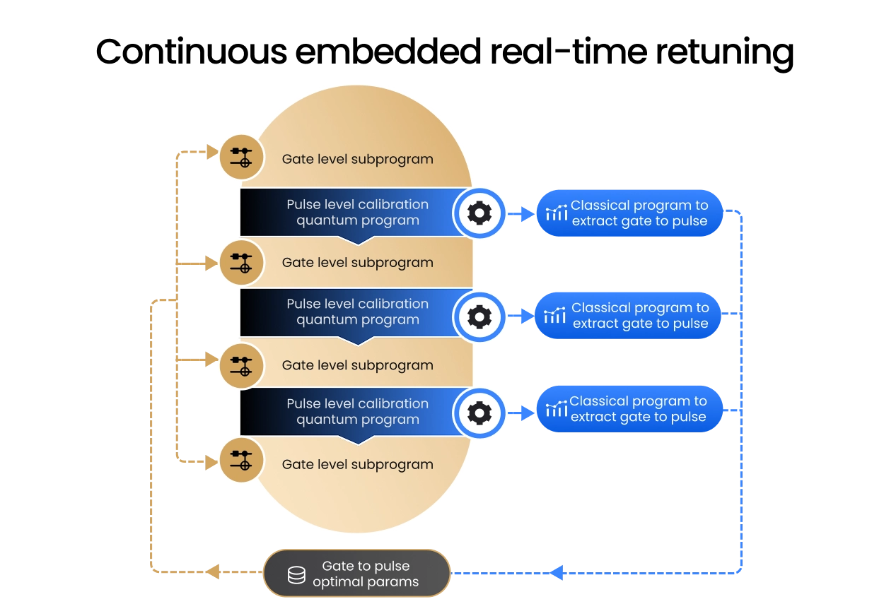
Instead of treating calibration as a separate offline step, quantum programs can call accelerated routines during execution, analyze measurement data in real time, and update pulse parameters, thresholds, frequencies, or control decisions before the next operation.
This enables fast drift tracking, adaptive tune-up, and experiment-aware calibration workflows that run alongside the quantum workload and respond to the system needs in real-time. It is the infrastructure needed for large-scale quantum processors: quantum control, calibration logic, and classical acceleration operating as one real-time system.
“Dedicated hardware for controlling and operating quantum bits is something we have all been dreaming of. Quantum Machines has answered this call by allowing us and others in the field to scale up with ease and with far greater functionality than was ever possible before. “
Prof. Amir Yacoby
Professor
“OPX has been a powerful enabler in our lab, helping us quickly characterize the performance of our recently discovered qubits. The hardware removes time wasted in uploading and waiting during pulse programming. QUA has substantially reduced the complexity of writing quantum protocols, allowing us to code dynamical decoupling and RB sequences in just a few lines. It remarkably saves our time in optimizing the processes and visualizing the results, allowing us to focus more on understanding the physics of our new qubits.”
Prof. Dafei Jin
Professor
"OPX+ & Octave: Perfect, all-in-one measurement system for SNU's silicon 5 qubit device!"

Prof. Dohun Kim
Professor
“The OPX’s fast feedback and unique real-time processing capabilities were critical for our experiment. Combining these with the OPX’s intuitive programming and QM’s state-of-the-art cryogenic electronics allowed us to do something that we have dreamt of doing for years.”
Prof. Ferdinand Kuemmeth
Professor
Blog
Building the Strongest Link in the Quantum Stack: Welcoming Our Budapest Engineering Hub
Read more July 2026 | 6 min read
Blog
Quantum Machines’ Latest Acquisition Highlights Europe’s Growing Quantum Talent Base
Read more June 2026 | 4 min read
Scientific Publications
Loss Mechanisms in High-coherence Multimode Mechanical Resonators Coupled to Superconducting Circuits
Read more May 2026 | 1 min read
Scientific Publications
Learning Nonlinear Heterogeneity in Physical Kolmogorov-Arnold Networks
Read more May 2026 | 1 min readFAQ
How does QM’s platform scale spin-qubit controHow does the firmware preserve signal integrity across complex pulse sequences? l to large QPUs?
Digital filtering is implemented directly in firmware, with native FIR and IIR filters available for any pulse element: IIR filters compensate distortions from bias-tees, while FIR filters support sub-nanosecond baseband rise times and skew control at picosecond resolution. Because filtering runs on the PPU, pulse predistortion is applied in real time, which reduces memory use and shortens experiment run time. The same engine handles line-shape correction and synchronized timing across DC, RF, and readout channels.
How does QM manage crosstalk and DC offsets in dense gate arrays?
Crosstalk compensation matrices can be embedded in the configuration file, enabling real-time correction of capacitive coupling between adjacent gates as arrays get denser. For rapid, multidimensional voltage sequences, the system automatically generates compensation pulses to maintain zero net DC offset. The real-time engine also supports onboard PID loops for drift-sensitive charge sensors, with update rates of hundreds nanoseconds.
What is QuAM, and how does it simplify large-scale spin-qubit programming?
QuAM is an object-based representation of the QPU that lets quantum operations be parameterized at the qubit level, significantly reducing programming complexity for large processors. For spin qubits it lets users define their abstraction by target architecture — Loss-DiVincenzo, exchange-only, or singlet-triplet — and it incorporates shuttling architectures for multi-core QPUs. This makes calibration routines hardware-aware, reusable, and scalable rather than rewritten per device.
How does QUAlibrate automate spin-qubit tune-up at scale?
QUAlibrate turns QUA protocols and tuning routines into nodes of a calibration graph. The nodes can be covering gate virtualization, charge-stability scans, dot tuning, tunnel-rate calibration, Pauli-spin-blockade readout optimization, exchange calibration, and single- and two-qubit gate tune-up. These nodes can be automated, enriched with decision logic, and parallelized across many dots and qubits. Combined with QM’s Open Acceleration Stack, this integrates optimization and machine-learning workflows directly into the calibration loop for fast retuning and drift correction.