
Superconducting Qubits
Orchestrate superconducting-qubit experiments with precise microwave control, ultra-low-latency feedback, and embedded calibration workflows. Go from fast bring-up to adaptive circuits and scalable QPU operation with QM’s Orchestration Platform.


Research
Superconducting qubits are built from lithographically defined electrical circuits operated at millikelvin temperatures. Their quantum behavior arises from Josephson junctions and their nonlinear energy levels used to encode quantum information. This circuit-based approach has become one of the leading platforms for quantum computing, combining fast gate speeds, mature fabrication methods, and strong integration with hybrid control technology. Operating such circuits requires precise generation, synchronization, and measurements of microwave signals and baseband pulses. Additionally, advanced calibration routines and implementing quantum error correction require integration of heavy classical compute power, either within or in-between shots of quantum circuits.
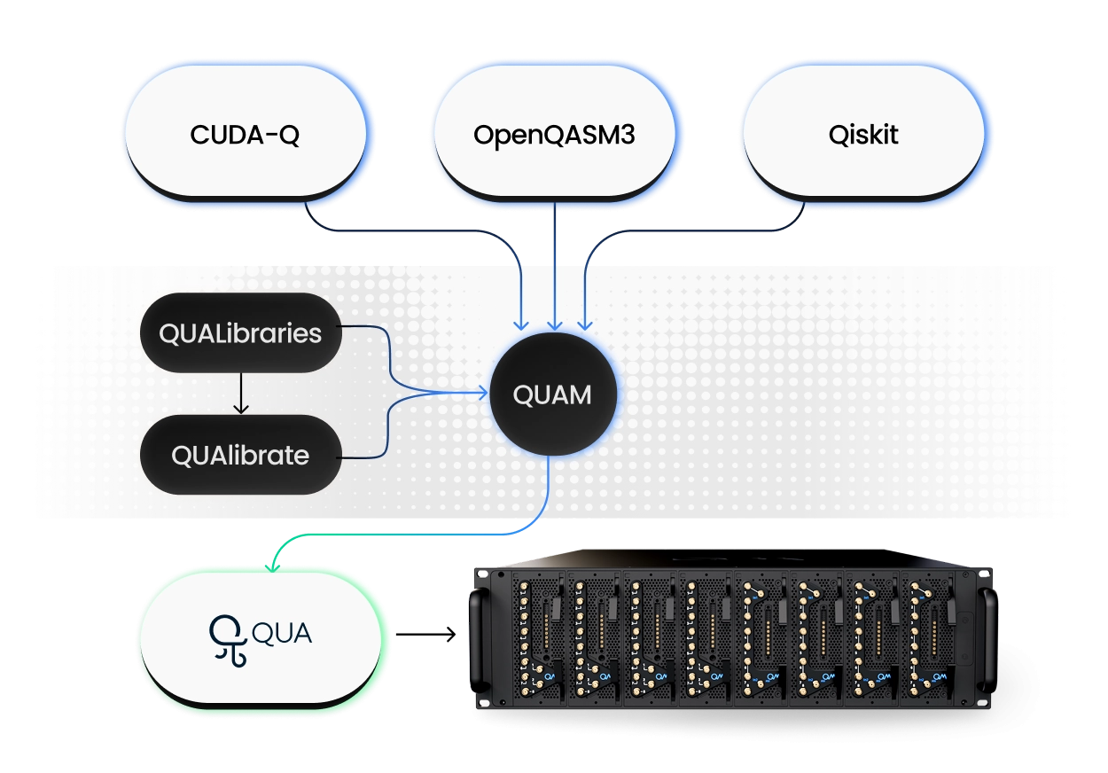
Quantum Machines’ Orchestration Platform supports the complete superconducting qubit workflow. The OPX1000 hybrid controller provides deterministic pulse timing, ultra-low latency feedback, and scalable orchestration across many channels, while integrating both baseband and microwave control and readout. With unmatched phase coherence and signal quality, fidelities reach new heights.
Powered by the Pulse Processing Unit, Quantum Machines’ control stack and its integration with classical accelerators via the Open Acceleration Stack, allow researchers to combine quantum operations with real time classical logic, enabling fast tune up, dynamic experiments, adaptive embedded calibrations, and real-time quantum error correction, which are all required features for scalable control of superconducting quantum processors.
Set Up Architecture
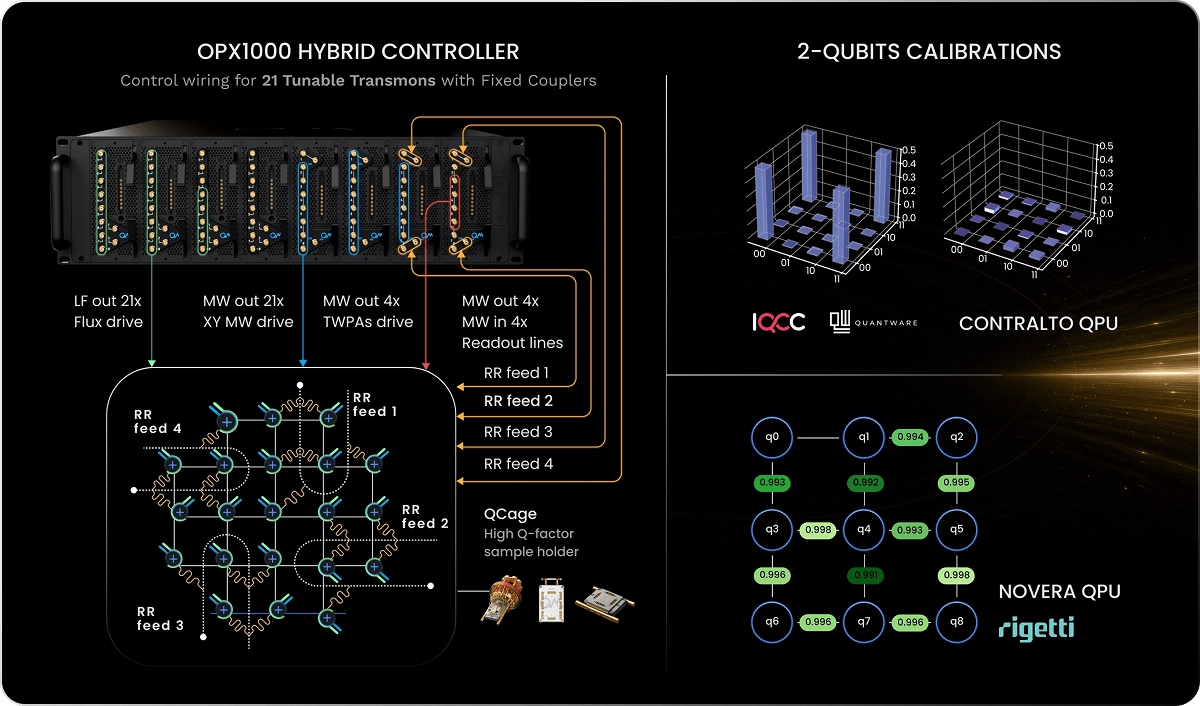
Quantum-Classical Integration and Control Highlights
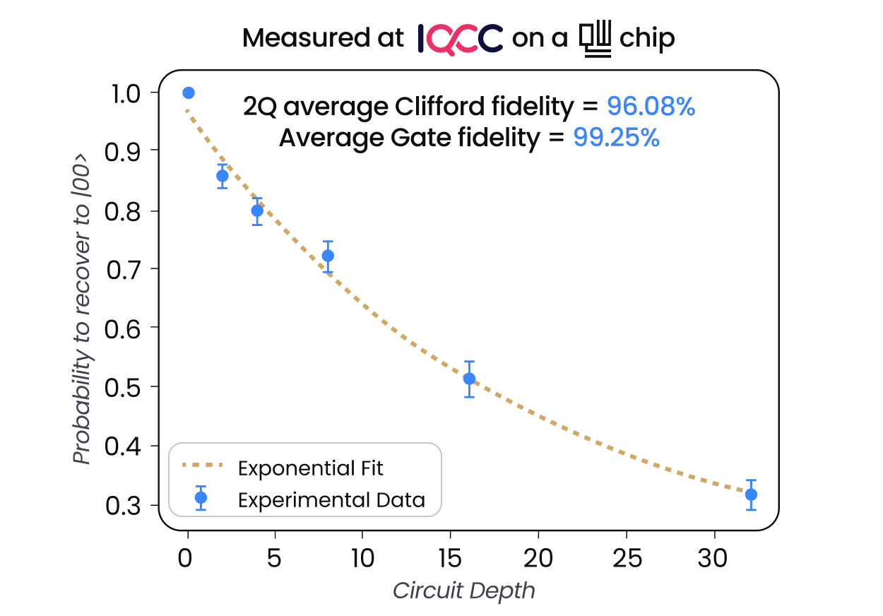
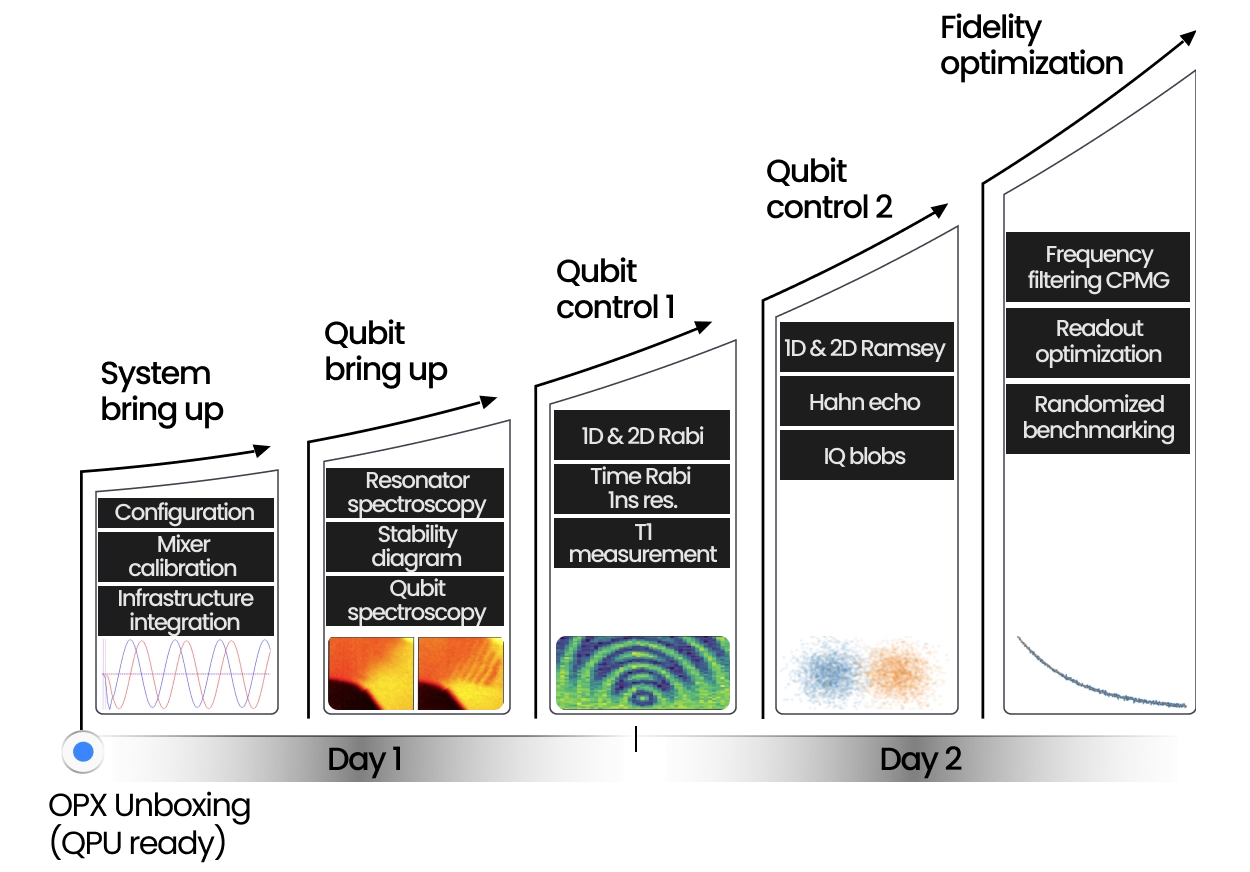
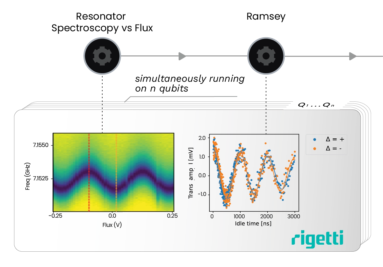
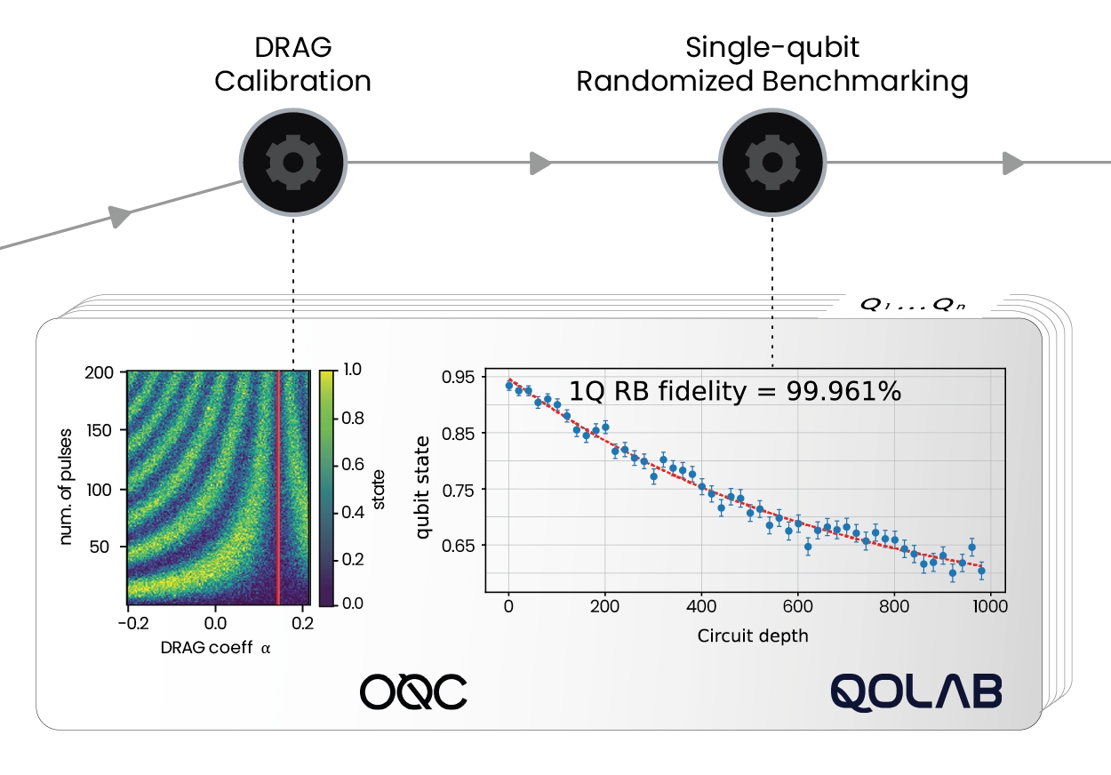
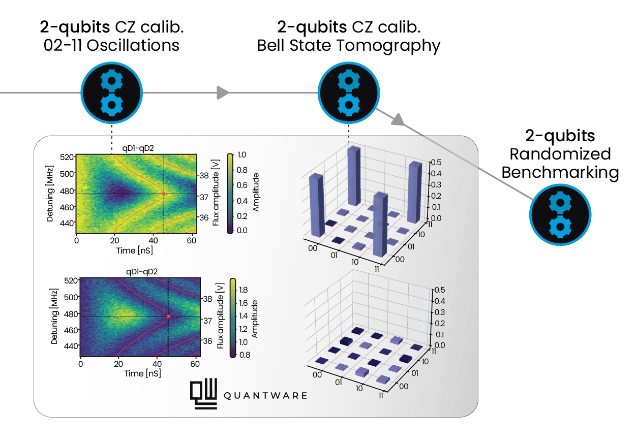
From Installation to 2-qubits Randomized Benchmarking in less than 48 hours
How long does it take to tune up and characterize your superconducting qubits starting from a brand-new controller? QM’s control suite powers hundreds of superconducting labs around the globe and shortens the path from plugging cables to two-qubit randomized benchmarking with stable, calibrated, high-fidelity operations.
Whether you work with fixed frequency, or tunable transmons, fluxonium qubits, dual-rail qubits, or any other superconducting device architecture, QM’s Orchestration Platform covers every need of qubit driving, readout, and fast analog feedback, including real-time computation and logic. Its OPX1000 Hybrid Controller generates parametric waveforms from DC to 10.5 GHz with direct digital synthesis (DDS), without any analog mixing, allowing for incredible signal purity, extensive multiplexing capabilities and bandwidth, and unparalleled phase stability. A single OPX1000 can handle multiple setups and experiments completely independently, allowing teams with multiple experimental tracks to use a single box to orchestrate the entire lab. Paired with the QCage, the purpose-built sample holder for superconducting devices, users benefit from optimal signal integration at the chip level and an ideal electromagnetic environment at millikelvin temperatures.
With the help of a QM Customer Success Physicist that visits you for the installation, setting up shop takes no time. The incredible expressiveness of QUA, our pulse-level programming language, makes discussing and writing sequences very intuitive. The vast repository of codes in our QUAlibs avoids reinventing the wheel. With hundreds of pre-coded experiments, from T1 to RB, DRAG calibration, frequency tracking, and more, progress is achieved on short timescales, and the typical installation and tune-up reaches 2-qubit Randomized Benchmarking within 2 days. This way you can start right away with your novel research endeavor, with QM at your side.
Real-time Control enabling Adaptive Quantum Circuits
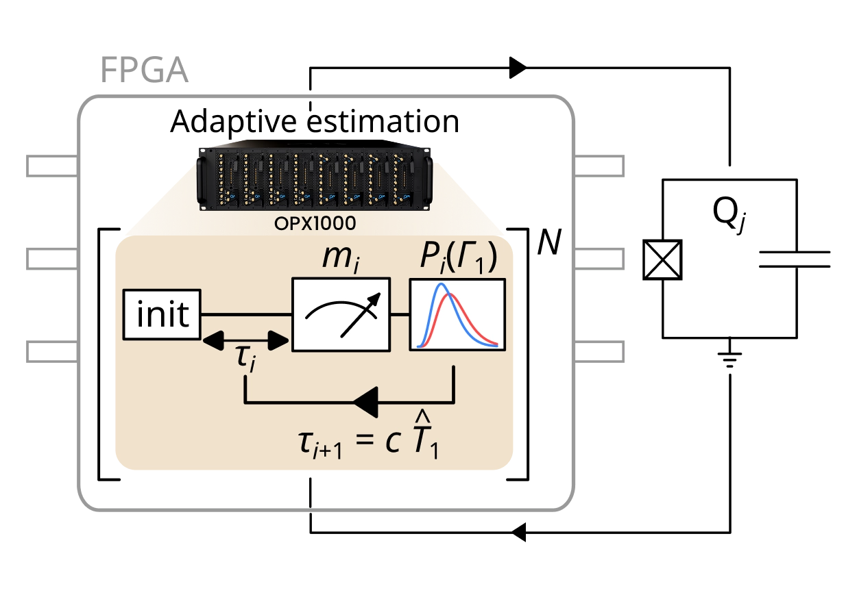
Quantum experiments increasingly require sequences that react while the physics is happening. At the simplest level, adaptive control can be boolean feedback, such as active reset: measure, decide, and apply a pulse only when needed. But the real frontier is richer control logic inside the sequence itself, where live measurement results can update parameters, choose the next pulse, branch between protocols, or run Bayesian estimations to decide the most informative next step.
QM’s Pulse Processing Unit makes this possible. Embedded in the OPX, the PPU is the first layer of classical integration within quantum sequences, combining precise quantum operations with real time computation and decision making. With the shortest feedback latency in the industry and highly varied compute capabilities, it turns the controller into an active part of the experiment.
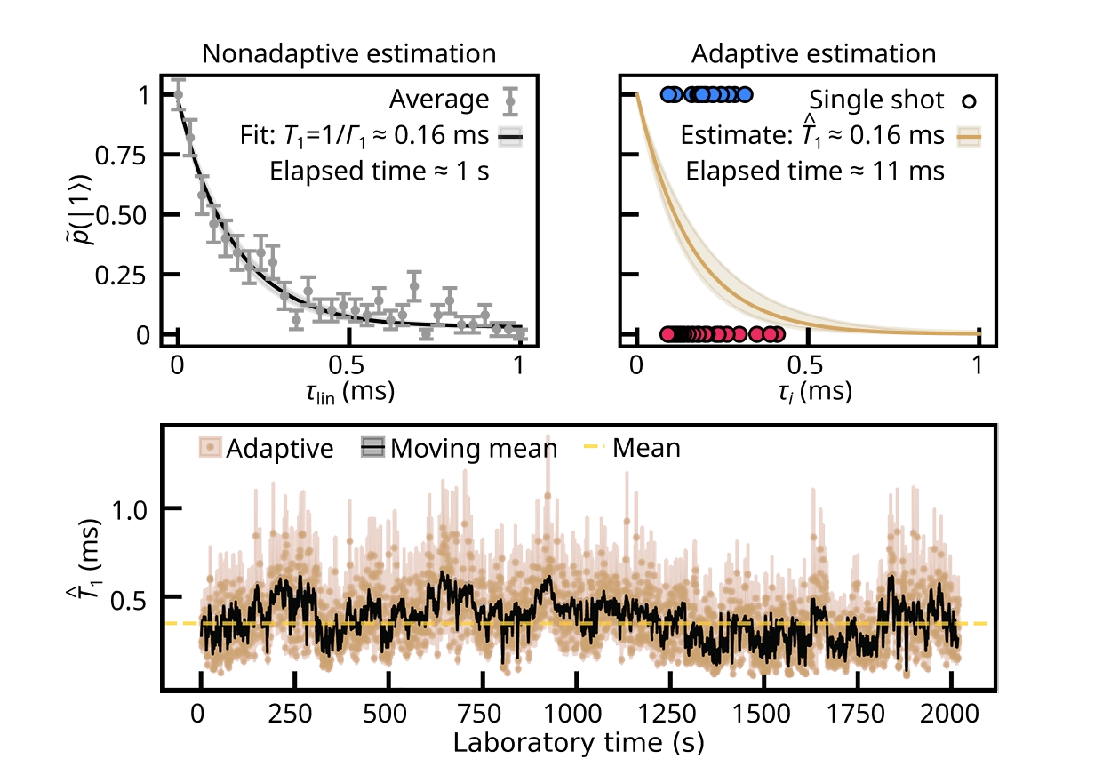
A recent superconducting qubit study [Berritta, F, et al. Physical Review X 16.1 (2026): 011025] showed the power of this approach, using real-time Bayesian estimation to reveal relaxation time fluctuations on millisecond time scales. In conventional measurement and analysis approaches, such dynamics are averaged away. For researchers, this tight integration of quantum and classical operations, opens the road to experiments that follow the system, expose hidden dynamics, and adapt to the QPU as it evolves. More generally, adaptability of programs with real-time compute capabilities allows to squeeze all the available information out of the interactions and measurements we subject our qubits to, and enables advanced embedded calibrations, smart handling of drifts and sequences, unique adaptive initialization techniques, and more.
Embedded Hybrid Calibrations with the Open Acceleration Stack
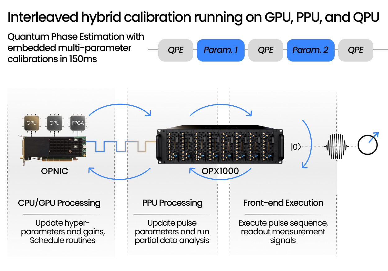
Long quantum workflows cannot rely on calibrations that happen only before circuit execution begins. QPUs are analog systems, meaning pulse amplitudes, frequencies, flux biases, and readout parameters can drift while an experiment is still running. While the OPX1000 and its Pulse Processing Unit enable fast adaptive calibration directly inside quantum sequences, the Open Acceleration Stack extends this further by integrating external classical accelerators into a low-latency loop.
With this hybrid architecture, the PPU can perform shot-to-shot feedback, while a CPU, GPU, or FPGA analyses the measurement history, updates hyperparameters, and schedules calibration routines between shots according to a predefined policy. The result is embedded calibration with accelerator processing in the 2-10 microsecond range, enabling multi-parameter full calibration workflows on roughly 100 millisecond timescales.
Phase estimation is a perfect example of this capability. When qubit flux and frequency drift freely, the extracted phase becomes unstable and can converge to the wrong value. By interleaving the main circuit with targeted calibration nodes, the system keeps readout, flux, frequency, and pulse amplitudes locked throughout execution. Faster drifting parameters can be calibrated more often, while stable ones are updated less frequently.
This turns calibration from a separate maintenance step into a live, interleaved, automatic part of the quantum workflow. The computation keeps running while the control system continuously uses the measurements already being collected to decide how to preserve performance in real time.


QM's control electronics provide the best real-time features along with an intuitive and well-documented programming interface. At TII, we successfully controlled a 25-q chip and conducted multiplexed characterization of all qubits using QM’s OPX and Octave. What we appreciate most, however, is the QM’s unwavering support and commitment to helping us achieve our targets, even going so far as to send some of their best scientists when needed.

Alvaro Orgaz
Lead QC Control
Thanks to the super-fast on-board data processing of the OPX we could resolve the nonlinear phenomena of our superconducting quantum circuits. With conventional AWGs and electronics this would have taken an impractical long time. The OPX is extremely easy to operate and substantially changes the paradigm of data acquisition and analysis procedures in quantum labs.

Dr. Byoung-moo Ann
Researcher
The OPX makes developing a brand-new superconducting qubit capability from scratch a breeze. Getting started is straightforward, the coding is easy, and the customer support is fantastic! The OPX reduces the potential barrier to progress and is also well suited for teaching.

Dr. Christian Boutan
Researcher
I must say I'm very happy with QM's Quantum Orchestration Platform. It's the single most reliable piece of equipment I've got in the lab. I operate it remotely and never had any problems. I strongly recommend the OPX and the QOP to my colleagues. It is by far the simplest way to do qubit physics.

Dr. Emmanuel Flurin
Researcher
Using high-fidelity rapid readout and real-time state assignment, we were able to do an active reset and generate this noiseless plot (100,000 times averaging) in 20 seconds. Without active reset (assuming 400us between sequences) it would have taken roughly an hour to get a similar quality plot.” Dr. Eunjong Kim Painter Lab, Institute for Quantum Information and Matter (IQIM), Caltech Simultaneous control and reset at scale – 10-qubit device example X180

Dr. Eun Jong Kim
Researcher
With the OPX we were able to reduce the cost of infrastructure development from a few weeks to a few days, without any need to directly program the FPGA.

Dr. Roni Winik
Engineering Quantum System Group
Quantum Machines' OPX played a key role in our roadmap. It enabled us to get the best control electronics out there [FPGA] without having to learn how to program them. QM provides a very scalable, very easy to use and very powerful hardware, which allows us to focus on the quantum science.

Dr. Théau Peronnin
CEO u0026 Co-Founder
Having tried several instruments in the past, I am very impressed by Quantum Machines' OPX. It finally removes the need for us to develop any skills in FPGA programming while still benefiting from advanced FPGA capabilities in our experiments.

Prof. Benjamin Huard
Professor
The OPX+ has allowed us to tune up complex multi-qubit measurements with multiplexed control and readout signals for studying quasiparticle poisoning and correlated errors in superconducting qubit arrays. The on-board processing has been quite useful for analyzing qubit data streams on the fly.

Prof. Britton Plourde
Professor
OPX has been a powerful enabler in our lab, helping us quickly characterize the performance of our recently discovered qubits. The hardware removes time wasted in uploading and waiting during pulse programming. QUA has substantially reduced the complexity of writing quantum protocols, allowing us to code dynamical decoupling and RB sequences in just a few lines. It remarkably saves our time in optimizing the processes and visualizing the results, allowing us to focus more on understanding the physics of our new qubits.
Prof. Dafei Jin
Professor
Developing a functional Qubit control electronic system absorbs a PhD-student full time at least for 2 years. QM’S Quantum Orchestration Platform allowed us set up experiments for full Qubit characterization in

Prof. Gerhard Kirchmair
Professor
We are very pleased with the QOP control solution. It’s remarkably easy to use, reliable, and flexible, supporting our advanced quantum research needs. The QOP dramatically expedites our research. Moreover, the Quantum Machines customer team has been instrumental in addressing all our needs to help us to maximize the full potential of the solution. We already use two systems and strongly recommend it.

Prof. Eli Levenson-Falk
Professor
QCage integrates seamlessly into our workflow of preparing and loading QPUs and supports higher throughput in our lab. Our research directly benefits from QCage's innovative design and engineering.

Prof. Javad Shabani
OPX played a crucial role in our advanced quantum experiments. This platform is the most flexible and user-friendly system in our lab. It saved us a significant amount of time, enabling us to concentrate on quantum science and make progress much faster compared to writing our own code. Furthermore, the Quantum Machines customer success team has been extremely helpful in addressing our needs and maximizing the solution's full potential.

Prof. Johannes Fink
Professor
My group is completely satisfied with the multiple OPX systems we’ve purchased. Qubit bring-up is fast and easy, as is optimization of high-fidelity microwave and z-pulse gates. The technical support team at Quantum Machines is outstanding.

Prof. Robert F. McDermott
Professor
The OPX+ and Octave are a dramatic improvement over the traditional homemade AWG plus DAQ systems. These QM instruments offer ease of use across several levels of abstraction: from implementing and optimizing individual pulses to realizing complex experiments with real time processing and feedback. Coding is user-friendly, which makes transmitting the know-how between group members much more straightforward.

Prof. Sorin Paraoanu
Associate Professor

Blog
Blog
Quantum Machines’ Latest Acquisition Highlights Europe’s Growing Quantum Talent Base
Read more June 2026 | 4 min read
Scientific Publications
Loss Mechanisms in High-coherence Multimode Mechanical Resonators Coupled to Superconducting Circuits
Read more May 2026 | 1 min read
Scientific Publications
Learning Nonlinear Heterogeneity in Physical Kolmogorov-Arnold Networks
Read more May 2026 | 1 min readFAQs
What distinguishes an integrated quantum orchestration platform in superconducting systems?
An integrated orchestration platform unifies waveform generation, timing, measurement, and classical compute in one deterministic backbone, unlike modular stacks such as that require layered integration. In the OPX1000, all the steps from acquiring the waveform, to analyzing it, manipulating it and then performing control logic on it happens on the same controller ensuring minimal latency and deterministic performance. The open acceleration stack further extends these capabilities by enabling seamless interfacing with external servers via OPNIC, unlocking advanced computational workflows and expanding the scope of real-time and offline processing.
How does the control platform enable high parallelism?
High‑parallelism quantum control requires precise synchronization across many control lines. The OPX1000 enables this by performing waveform generation, signal acquisition, real‑time analysis, manipulation, and control logic execution all within a single controller.
Because the full control loop runs locally on the same unit, parallelism does not require splitting functionality across multiple boxes. Scaling is achieved simply by scaling up the OPX1000 itself. When higher channel counts are needed, multiple OPX1000 units can be clustered into a single, time‑coherent system, synchronized via a shared clocking architecture and low‑latency optical links.
This unified architecture minimizes latency, avoids signal‑path matching, and enables deterministic, highly parallel multi‑qubit control at scale.
How does architecture choice impact long-term roadmap viability?
As superconducting systems scale toward thousands of qubits and continuous error correction, only integrated orchestration architectures remain viable. Real‑time QEC requires mid‑circuit measurement, active reset, and conditional control within <200 ns; any architecture that relies on host‑side decisions introduces >1 ms latency and cannot meet these budgets.
The OPX1000, together with QUA, QUAM, and the Open Acceleration Stack, provides the structured QPU hardware model required by QEC orchestration layers and classical decoders to construct syndrome extraction circuits, assign decoder weights, and adapt to measured qubit parameter drift over time. This enables deterministic mid‑circuit control, repeat‑until‑success protocols, and scalable stabilization cycles, making the platform aligned with long‑term fault‑tolerant quantum roadmaps.
Can superconducting qubits support fault-tolerant quantum computing?
Yes, superconducting qubits are promising as they scale from 25 qubits today to 100, 500, and ultimately to fault-tolerant operation. Quantum Machines’ OPX1000 was built to support every stage of it, including demonstrated capabilities of simultaneous, sub-second calibration of dozens of qubits with minimal overhead, and low-latency GPU/CPU integration required for QEC. What sets the platform apart is not channel count & density or analog performance alone, but the unification of classical computation and quantum control across the full stack from real-time hardware-level processing through software orchestration to classical accelerator and HPC-level workflows. This is Quantum Machines’ core mission: the full orchestration of classical and quantum computation, at every layer of the stack.
Why is low-latency feedback critical for superconducting error correction?
Quantum programs require tightly interleaved quantum and classical operations. Classical compute latency must match the short timescales of the quantum system, while also scaling with increasing qubit counts.
In Quantum Machines’ OPX1000, each module is powered by a Pulse Processing Unit (PPU) capable of executing classical operations such as arithmetic, variable updates, comparisons, and control flow directly within the same real-time execution timeline as pulse generation and measurement, with nanosecond-scale waveform resolution and sequencing granularity.
This tight integration enables deterministic, low-latency feedback essential for stabilizing quantum states and implementing error correction protocols.
What limits coherence time in superconducting qubits?
Coherence in superconducting qubits is degraded by a variety of factors like flux noise, charge noise, dielectric loss, and quasiparticle poisoning, and material defects. All of these cause qubit frequencies, gate parameters and readout fidelity to drift during extended sequences. In the OPX1000, the PPU’s embedded calibration routines track and correct frequency drift mid-experiment in real time, without halting execution or requiring operator intervention.
What limits two-qubit gate fidelity in superconducting systems?
Two-qubit gate fidelity is limited by residual ZZ coupling, leakage to non-computational states, microwave crosstalk, and coupler calibration drift. Because two-qubit gates are slower than single-qubit operations, they are more exposed to decoherence during execution. The OPX1000 addresses this through ultra-low-latency feedback and real-time pulse corrections, keeping gate operations within the coherence budget.
Scale
Scaling superconducting quantum processors requires more than adding qubits. As systems grow, every layer of control must scale with them, from synchronized microwave and baseband pulse generation to automated tune up, high fidelity gate calibration, multiplexed readout, and real time integration with classical compute. Achieving and maintaining performance across larger devices requires continuous calibrations, fast optimization, and precise correction of signal distortions throughout the scaled-up chain.
Quantum Machines’ Orchestration Platform is built to support this transition from device operation to scalable quantum processing. The OPX1000 hybrid controller provides deterministic timing, phase coherent control, low latency feedback, and scalable orchestration across dense multiqubit systems without compromises. Signal integrity and digital filters allow for unmatched operational fidelity and two-qubits gates calibrations.
Such high fidelity must be maintained across minutes and hours of operation. At scale, calibration becomes a central challenge. QUAlibrate enables automated, structured, and repeatable calibration workflows that help teams tune large systems efficiently and maintain device performance over time. Advanced characterization routines, allow researchers to identify and compensate for distortions and drifts that limit gate fidelity, for an industry-level hands-off routine that keeps QPU utilization high.
Powered by the Pulse Processing Unit and integrated with classical accelerators through the Open Acceleration Stack, Quantum Machines’ control architecture enables real-time quantum error correction decoding and adaptive calibration workflows. This creates a unified path toward reliable, high fidelity, and scalable superconducting quantum processors.
Set Up Architecture
Quantum-Classical Integration and Control Highlights
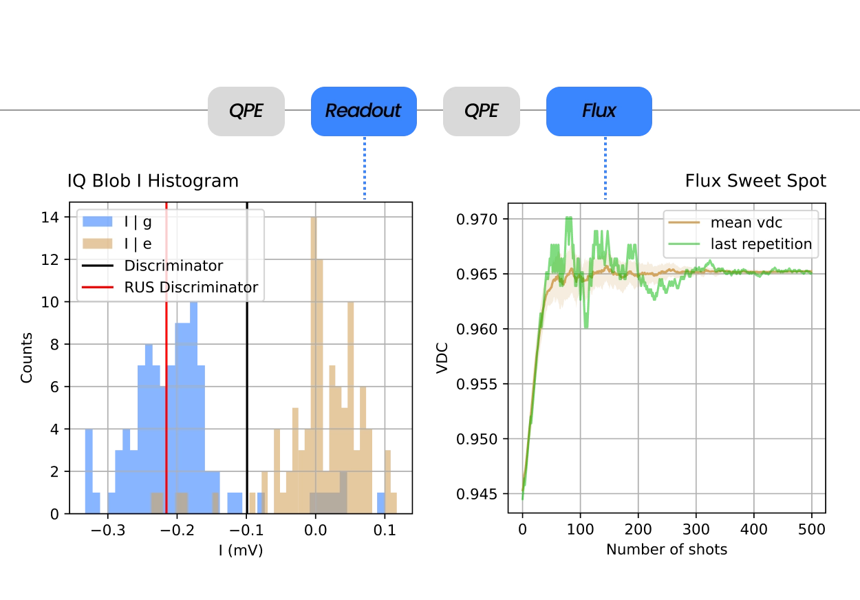
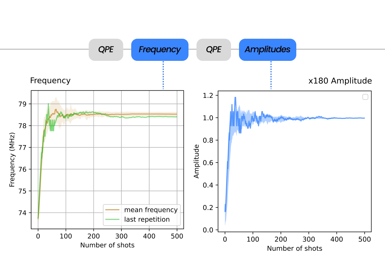
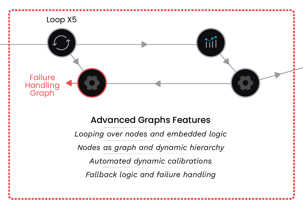
Keeping Fidelities High with Automated Calibrations
Tuneup and characterization of your qubits is not the end of the story. With time, parameters drift, optimal operation points move, and fidelities plummet. Thanks to QM’s Orchestration Platform, keeping systems operational becomes a fast and automated process.
QUAlibrate, QM’s free software for automated calibrations, takes your QUA protocols and tuning routines and turns them into nodes of a calibration graph. Graphs can be automated, imbued with additional logic, and parallelized over any number of qubits. With QM’s Open Acceleration Stack graphs can include reinforcement learning agents on CPU/GPU to take part in the more complex or large-scale calibrations. Advanced graph logic allows further optimization of the calibration process, failure handling, graph loops, and more.
QM’s QUAlibs includes a plethora of calibration graphs and nodes optimized for different systems or drifts, so you never need to start from scratch. This includes calibration routines for commercially available chips, such as Quantware, Rigetti, Qolab, and more, all currently available to use via cloud thanks to the Israeli Quantum Computing Center, powered by Quantum Machines. Whether you have 5 or 500 qubits, the retuning of your quantum computing chips, both for single- and two-qubits gates, should not take longer than just a minute or two.
Reaching new fidelity heights with real-time correction of pulse distortions
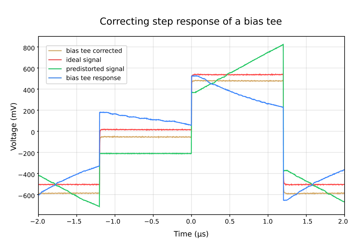
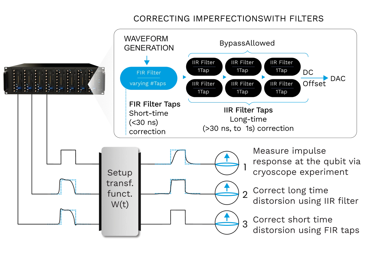
As superconducting processors grow toward hundreds of qubits, reaching high fidelity two-qubits gates across the chip becomes a major challenge. Flux tunable transmons require precisely shaped baseband pulses for entangling gates such as CZ, but by the time a waveform reaches the device it can be distorted by cables, attenuators, filters, bias tees, and skin effects. Ringing, overshoot, and slow tails shift the qubit frequency at the wrong moment and reduce gate fidelity.
Cryoscope and Digital Filters close this loop. A Cryoscope experiment turns each qubit into an in-situ oscilloscope, using Ramsey style interferometry to reconstruct the flux seen on chip with nanosecond resolution. Quantum Machines embeds these routines in QUAlibrate as automated nodes. One captures fast distortions and computes FIR feedforward taps at 2 GSa/s on OPX1000. The other uses qubit spectroscopy to resolve slower exponential drifts above 30 ns, fitting up to six decays and configuring IIR filters with time constants from 1 ns to 1 s.
Together, OPX1000’s DDS technology and these correction routines reduce flux pulse errors below 0.1% across the full range. The result is a pulse that reaches the chip exactly as programmed, making precise two-qubits calibration tractable as systems scale, and making the system ready for Quantum Error Correction (QEC).
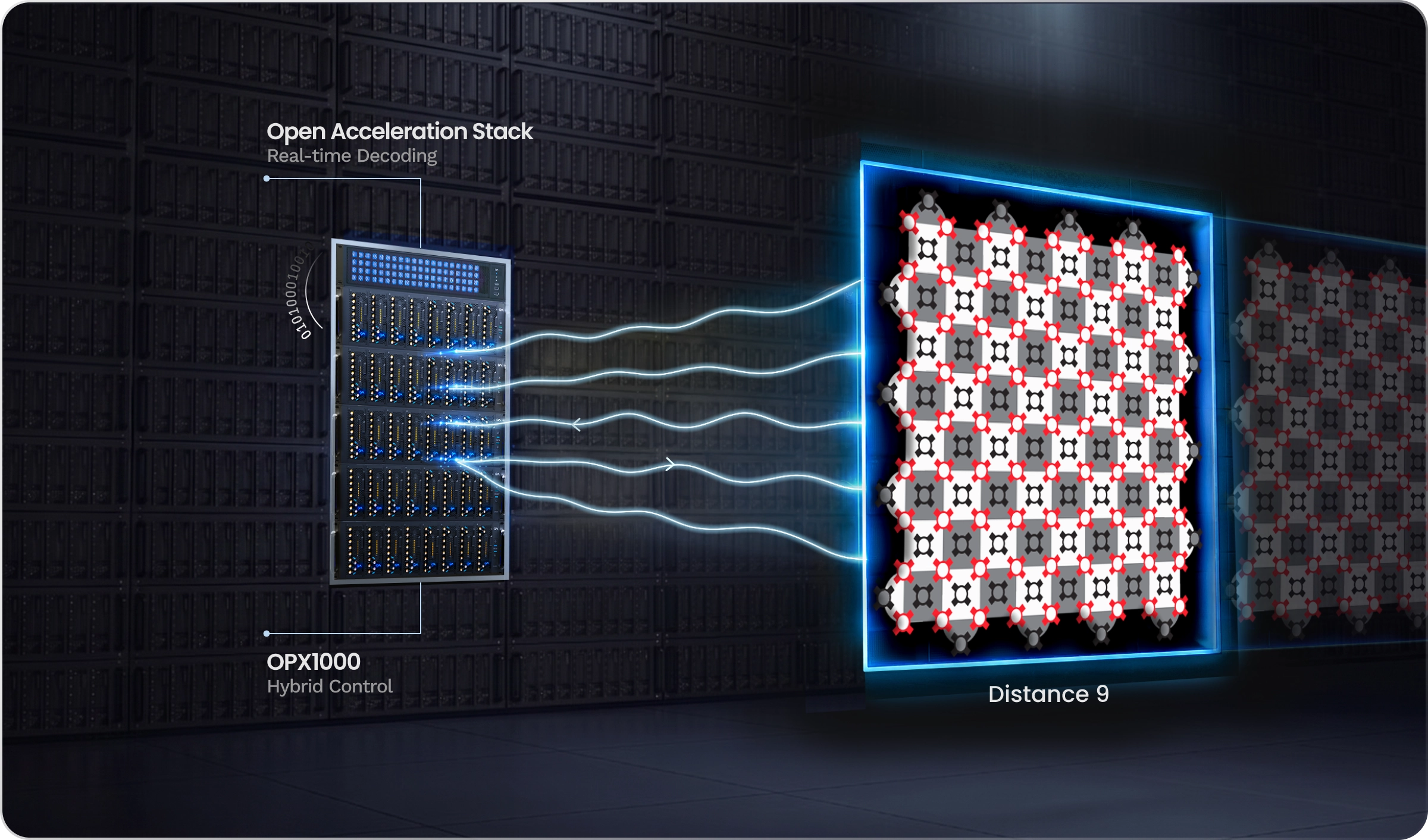
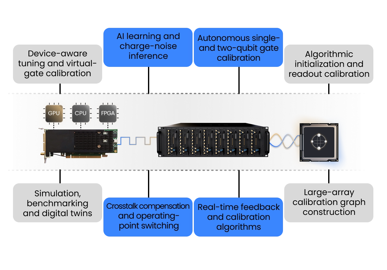
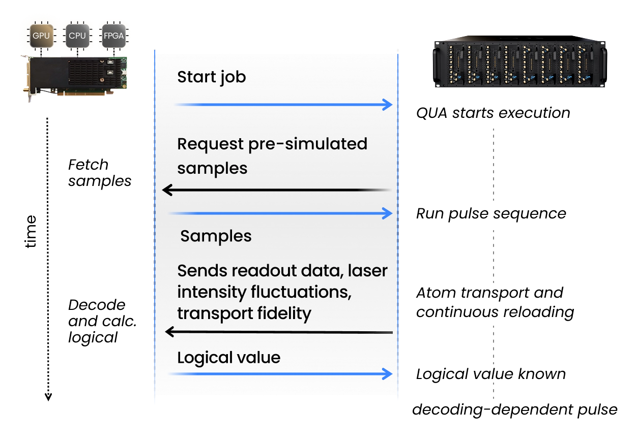
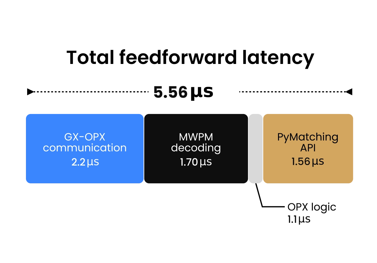
Real Time QEC with QM’s Open Acceleration Stack
Fault tolerant superconducting processors require real time decoding, feed-forward, and classical decisions inside every shot. QM’s Open Acceleration Stack connects the OPX1000 to external CPUs, GPUs, and FPGAs through low latency links, allowing a quantum sequence to call a decoder or accelerator and apply the result immediately as the next pulse.
To demonstrate the power of real-time QEC decoders on accelerators, we executed an error corrected quantum phase estimation workflow as a typical non Clifford circuit, including repeat until success angle injection, fault tolerant measurements, and decoding dependent feed-forward.
OPX1000 choses the decoding path in real time: simple cases were handled locally in the PPU, while harder syndromes were sent to an external MWPM decoder. This enabled 264 ns internal decoding and <3 microsecond external decoding latency, including communication and processing.
This is the infrastructure needed for QEC at scale: quantum control, decoding, and classical acceleration working as one real time system.
QM's control electronics provide the best real-time features along with an intuitive and well-documented programming interface. At TII, we successfully controlled a 25-q chip and conducted multiplexed characterization of all qubits using QM’s OPX and Octave. What we appreciate most, however, is the QM’s unwavering support and commitment to helping us achieve our targets, even going so far as to send some of their best scientists when needed.
Alvaro Orgaz
Lead QC Control
Thanks to the super-fast on-board data processing of the OPX we could resolve the nonlinear phenomena of our superconducting quantum circuits. With conventional AWGs and electronics this would have taken an impractical long time. The OPX is extremely easy to operate and substantially changes the paradigm of data acquisition and analysis procedures in quantum labs.
Dr. Byoung-moo Ann
Researcher
The OPX makes developing a brand-new superconducting qubit capability from scratch a breeze. Getting started is straightforward, the coding is easy, and the customer support is fantastic! The OPX reduces the potential barrier to progress and is also well suited for teaching.
Dr. Christian Boutan
Researcher
I must say I'm very happy with QM's Quantum Orchestration Platform. It's the single most reliable piece of equipment I've got in the lab. I operate it remotely and never had any problems. I strongly recommend the OPX and the QOP to my colleagues. It is by far the simplest way to do qubit physics.
Dr. Emmanuel Flurin
Researcher
Using high-fidelity rapid readout and real-time state assignment, we were able to do an active reset and generate this noiseless plot (100,000 times averaging) in 20 seconds. Without active reset (assuming 400us between sequences) it would have taken roughly an hour to get a similar quality plot.” Dr. Eunjong Kim Painter Lab, Institute for Quantum Information and Matter (IQIM), Caltech Simultaneous control and reset at scale – 10-qubit device example X180
Dr. Eunjong Kim
Researcher
With the OPX we were able to reduce the cost of infrastructure development from a few weeks to a few days, without any need to directly program the FPGA.
Dr. Roni Winik
Engineering Quantum System Group
Quantum Machines' OPX played a key role in our roadmap. It enabled us to get the best control electronics out there [FPGA] without having to learn how to program them. QM provides a very scalable, very easy to use and very powerful hardware, which allows us to focus on the quantum science.
Dr. Théau Peronnin
CEO u0026 Co-Founder
Having tried several instruments in the past, I am very impressed by Quantum Machines' OPX. It finally removes the need for us to develop any skills in FPGA programming while still benefiting from advanced FPGA capabilities in our experiments.
Prof. Benjamin Huard
Professor
The OPX+ has allowed us to tune up complex multi-qubit measurements with multiplexed control and readout signals for studying quasiparticle poisoning and correlated errors in superconducting qubit arrays. The on-board processing has been quite useful for analyzing qubit data streams on the fly.
Prof. Britton Plourde
Professor
OPX has been a powerful enabler in our lab, helping us quickly characterize the performance of our recently discovered qubits. The hardware removes time wasted in uploading and waiting during pulse programming. QUA has substantially reduced the complexity of writing quantum protocols, allowing us to code dynamical decoupling and RB sequences in just a few lines. It remarkably saves our time in optimizing the processes and visualizing the results, allowing us to focus more on understanding the physics of our new qubits.
Prof. Dafei Jin
Professor
Developing a functional Qubit control electronic system absorbs a PhD-student full time at least for 2 years. QM’S Quantum Orchestration Platform allowed us set up experiments for full Qubit characterization in
Prof. Gerhard Kirchmair
Professor
We are very pleased with the QOP control solution. It’s remarkably easy to use, reliable, and flexible, supporting our advanced quantum research needs. The QOP dramatically expedites our research. Moreover, the Quantum Machines customer team has been instrumental in addressing all our needs to help us to maximize the full potential of the solution. We already use two systems and strongly recommend it.
Prof. Eli Levenson-Falk
Professor
QCage integrates seamlessly into our workflow of preparing and loading QPUs and supports higher throughput in our lab. Our research directly benefits from QCage's innovative design and engineering.
Prof. Javad Shabani
OPX played a crucial role in our advanced quantum experiments. This platform is the most flexible and user-friendly system in our lab. It saved us a significant amount of time, enabling us to concentrate on quantum science and make progress much faster compared to writing our own code. Furthermore, the Quantum Machines customer success team has been extremely helpful in addressing our needs and maximizing the solution's full potential.
Prof. Johannes Fink
Professor
My group is completely satisfied with the multiple OPX systems we’ve purchased. Qubit bring-up is fast and easy, as is optimization of high-fidelity microwave and z-pulse gates. The technical support team at Quantum Machines is outstanding.
Prof. Robert F. McDermott
Professor
The OPX+ and Octave are a dramatic improvement over the traditional homemade AWG plus DAQ systems. These QM instruments offer ease of use across several levels of abstraction: from implementing and optimizing individual pulses to realizing complex experiments with real time processing and feedback. Coding is user-friendly, which makes transmitting the know-how between group members much more straightforward.
Prof. Sorin Paraoanu
Associate Professor
Blog
Building the Strongest Link in the Quantum Stack: Welcoming Our Budapest Engineering Hub
Read more July 2026 | 6 min read
Blog
Quantum Machines’ Latest Acquisition Highlights Europe’s Growing Quantum Talent Base
Read more June 2026 | 4 min read
Scientific Publications
Loss Mechanisms in High-coherence Multimode Mechanical Resonators Coupled to Superconducting Circuits
Read more May 2026 | 1 min read
Scientific Publications
Learning Nonlinear Heterogeneity in Physical Kolmogorov-Arnold Networks
Read more May 2026 | 1 min readFAQs
What distinguishes an integrated quantum orchestration platform in superconducting systems?
An integrated orchestration platform unifies waveform generation, timing, measurement, and classical compute in one deterministic backbone, unlike modular stacks such as that require layered integration. In the OPX1000, all the steps from acquiring the waveform, to analyzing it, manipulating it and then performing control logic on it happens on the same controller ensuring minimal latency and deterministic performance. The open acceleration stack further extends these capabilities by enabling seamless interfacing with external servers via OPNIC, unlocking advanced computational workflows and expanding the scope of real-time and offline processing.
How does the control platform enable high parallelism?
High‑parallelism quantum control requires precise synchronization across many control lines. The OPX1000 enables this by performing waveform generation, signal acquisition, real‑time analysis, manipulation, and control logic execution all within a single controller.
Because the full control loop runs locally on the same unit, parallelism does not require splitting functionality across multiple boxes. Scaling is achieved simply by scaling up the OPX1000 itself. When higher channel counts are needed, multiple OPX1000 units can be clustered into a single, time‑coherent system, synchronized via a shared clocking architecture and low‑latency optical links.
This unified architecture minimizes latency, avoids signal‑path matching, and enables deterministic, highly parallel multi‑qubit control at scale.
How does architecture choice impact long-term roadmap viability?
As superconducting systems scale toward thousands of qubits and continuous error correction, only integrated orchestration architectures remain viable. Real‑time QEC requires mid‑circuit measurement, active reset, and conditional control within <200 ns; any architecture that relies on host‑side decisions introduces >1 ms latency and cannot meet these budgets.
The OPX1000, together with QUA, QUAM, and the Open Acceleration Stack, provides the structured QPU hardware model required by QEC orchestration layers and classical decoders to construct syndrome extraction circuits, assign decoder weights, and adapt to measured qubit parameter drift over time. This enables deterministic mid‑circuit control, repeat‑until‑success protocols, and scalable stabilization cycles, making the platform aligned with long‑term fault‑tolerant quantum roadmaps.
Can superconducting qubits support fault-tolerant quantum computing?
Yes, superconducting qubits are promising as they scale from 25 qubits today to 100, 500, and ultimately to fault-tolerant operation. Quantum Machines’ OPX1000 was built to support every stage of it, including demonstrated capabilities of simultaneous, sub-second calibration of dozens of qubits with minimal overhead, and low-latency GPU/CPU integration required for QEC. What sets the platform apart is not channel count & density or analog performance alone, but the unification of classical computation and quantum control across the full stack from real-time hardware-level processing through software orchestration to classical accelerator and HPC-level workflows. This is Quantum Machines’ core mission: the full orchestration of classical and quantum computation, at every layer of the stack.
Why is low-latency feedback critical for superconducting error correction?
Quantum programs require tightly interleaved quantum and classical operations. Classical compute latency must match the short timescales of the quantum system, while also scaling with increasing qubit counts.
In Quantum Machines’ OPX1000, each module is powered by a Pulse Processing Unit (PPU) capable of executing classical operations such as arithmetic, variable updates, comparisons, and control flow directly within the same real-time execution timeline as pulse generation and measurement, with nanosecond-scale waveform resolution and sequencing granularity.
This tight integration enables deterministic, low-latency feedback essential for stabilizing quantum states and implementing error correction protocols.