
Neutral Atoms
Quantum Machines enables real-time orchestration across the neutral-atom stack, combining precise RF and optical control, synchronized gate operations, accelerated camera readout, and adaptive feedback for research and scale.


Research
Neutral atoms quantum computers have gained significant attention in recent years because they are naturally identical, can be rearranged with ease, and allow full optical control without the need for physical wiring. Quantum computers based on neutral atoms are based on a few simple steps: initialize a grid of atoms, perform gate operations, readout the state and repeat. In practice, however, each of these steps carries substantial latency rooted in both the underlying physics and the complexity of the control stack.
For neutral atoms, this means stable trapping, low‑loss transport, low‑latency readout, and precise individual control. Furthermore, running algorithms on them requires real‑time parallel processing and adaptive control such that circuit parameters and control flow update in real-time based on mid‑circuit measurements.
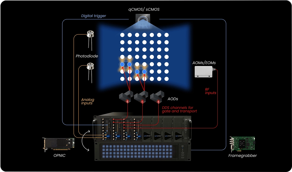
Quantum Machines’ OPX1000 allow for a wholistic solution by supporting multiple RF signals, flexible frequency-chirp patterns for atom motion, real-time updates based on camera data, and synchronized operation with gate control and readout, all under a globally synced timing reference.
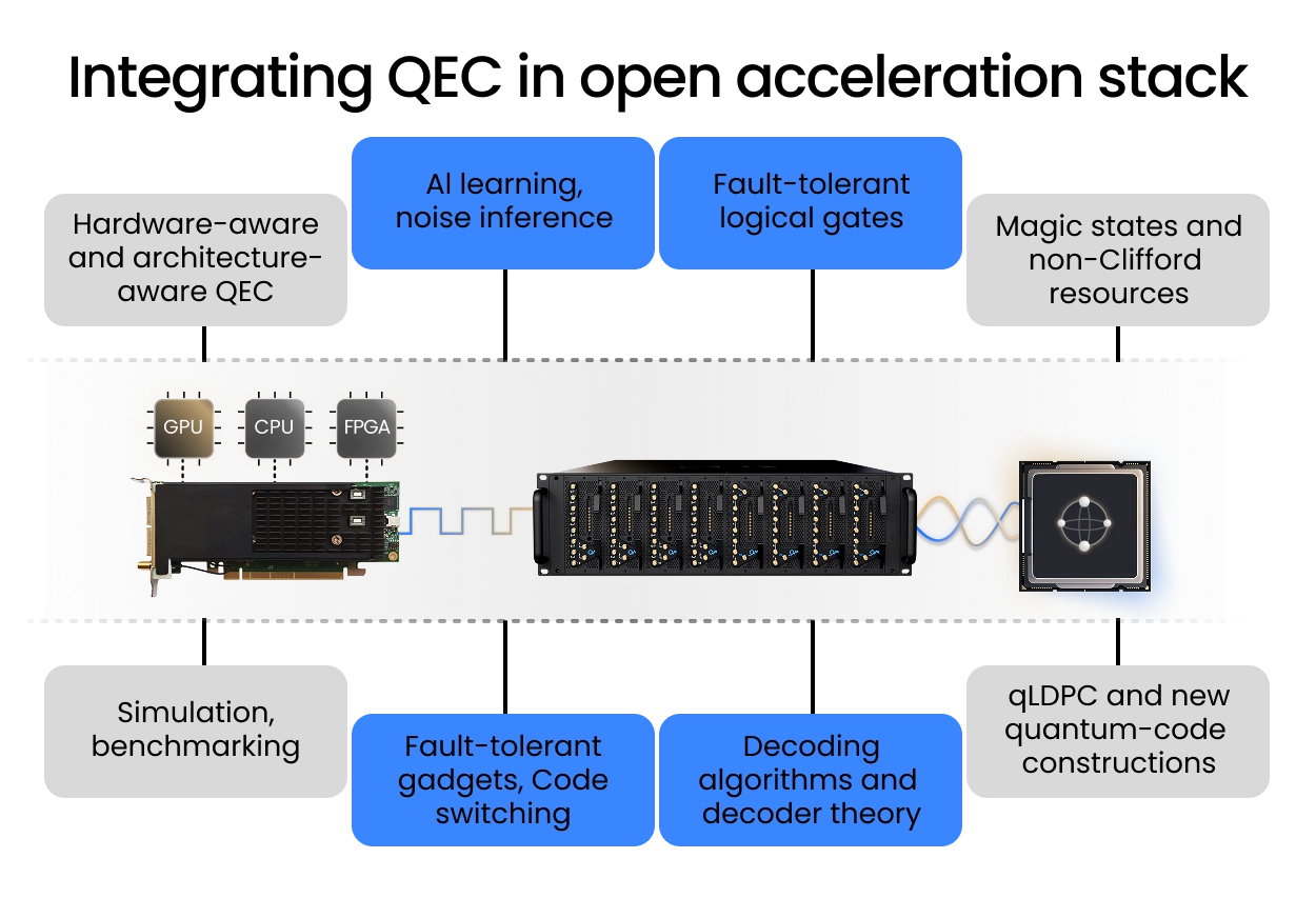
QUA, the OPX1000’s native pulse‑level language, enables true real‑time adaptive control by running concurrent processes like atom transport and reservoir refilling based on mid-circuit readouts directly on the controller. For scalers, the Quantum Machines’ OPNIC provides real-time interconnects, streaming results from the controller to a CPU/GPU server. The classical accelerators can be used to decode results and perform resource-heavy computations which can be then streamed back to the OPX1000 to update parameters.
Whether you’re controlling hundreds of atoms or scaling to thousands, QM’s solutions orchestrate the entire workflow, from sorting to gate operations, to readout, minimizing latency at every step so you can focus on the physics while we handle the control.
Set Up Architecture
Quantum-Classical Integration and Control Highlights
Real-time Atom Transport
A major advantage of neutral atoms is the ability to re-position and shuttle atoms around during the experiment. This makes it possible to change the configurations of the atoms and therefore allows for all-to-all connectivity and continuous reloading of atoms. This also enables unique capabilities, such as zone-based architectures and applying transversal gates.
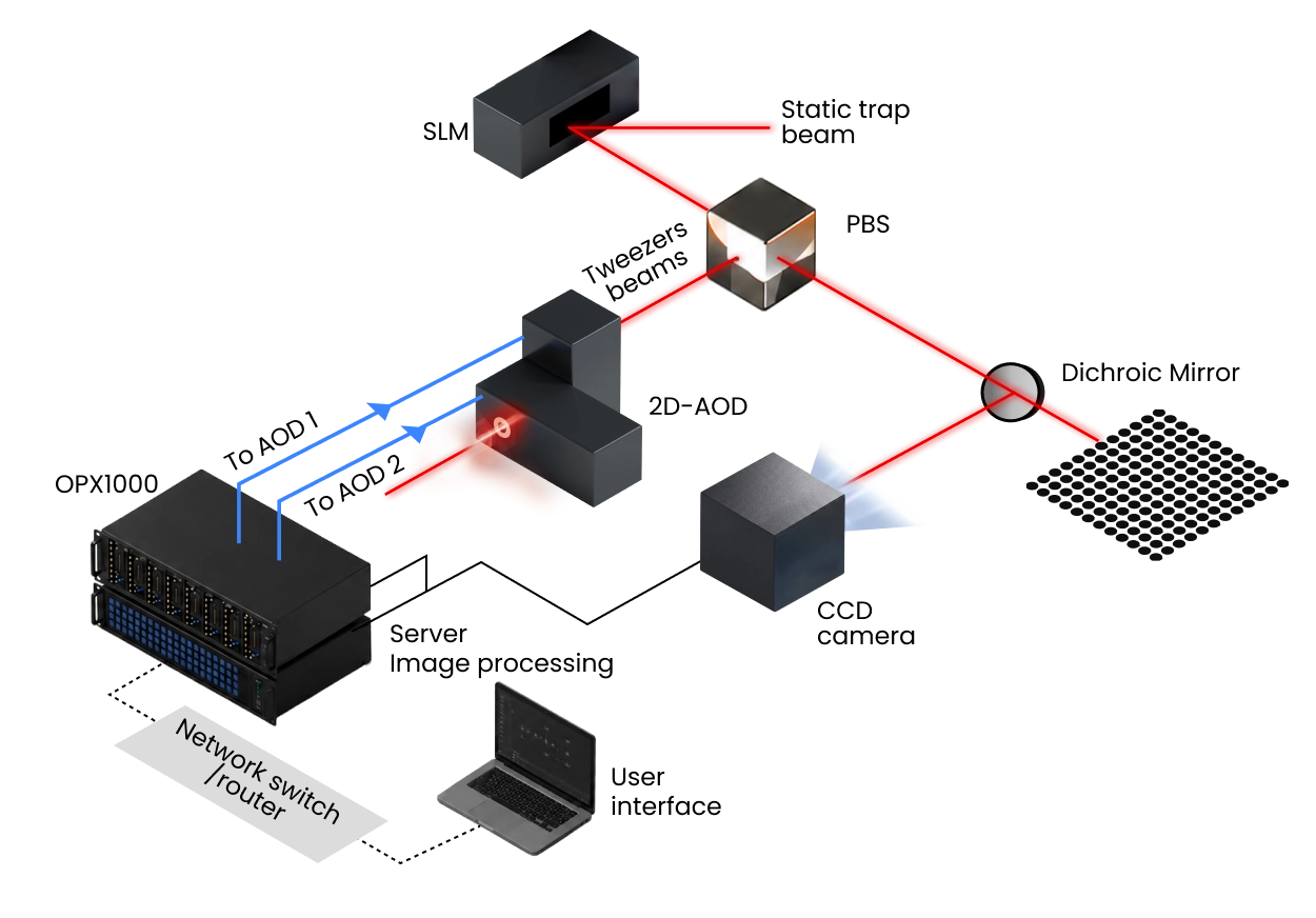
Standard architecture uses a spatial light modulator (SLM) to create a static array of optical tweezers, and a pair of crossed AODs (2D AOD) that are driven with RF tones to generate dynamic traps for atom transport.
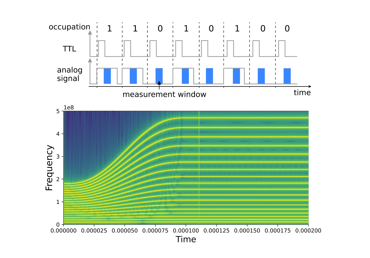
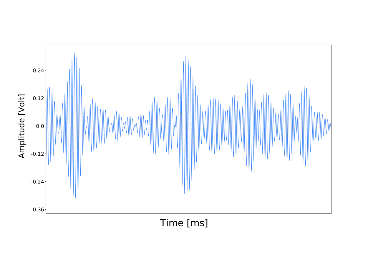
OPX1000 allow for a wholistic solution by supporting multiple RF signals, flexible frequency-chirp patterns for atom motion, real-time updates based on camera data, and synchronized operation with gate control and readout, all under a globally synced timing reference. To move atoms simultaneously and reconfigure large arrays, the OPX1000 provides multi-tone RF signals to the AOD, with each tone corresponding to a tweezer position. Rather than relying on large, pre-synthesized, waveform uploads, the core synthesizes waveforms on-the-fly, calculating the next segment while playing the current one. For more complex rearrangements, the user can provide precomputed arbitrary waveforms that can contain more frequency tones.
The Pulse level programming language QUA allows to seamlessly go from physical lab parameters like grid spacing to sophisticated rearrangement algorithms that efficiently transport atoms without losing them.
At Quantum Machines, we provide solutions for today and tomorrow. When scaling neutral atoms, the current solution can be insufficient. To achieve large-scale atom rearrangement with low latency, transport solutions must compute dynamically precisely shaped multi-tone AOD signals from readout images and routing algorithms. QM’s Open Acceleration Stack which connects the OPX1000 with classical CPU-GPU accelerators using the OPNIC allows for leveraging more classical compute power to address qubits with microsecond latency allowing for the solution to operate in quantum real time.
Gate Addressing and Orchestration
Neutral-atom quantum computing platforms use a variety of gate mechanisms. Common approaches to single-qubit gates include direct microwave driving or optical Raman transitions driven by two optical beams.
Typical two-qubit gates utilize Rydberg blockade to realize CZ gates using lasers. Laser pulses are shuttered and controlled through AOMs or electro-optic modulators (EOMs), which set the amplitude, phase, and frequency of the optical pulse. Single- and two-qubit gates can be driven by directly sending signals from OPX1000 to AOMs or to a microwave horn. For simple gates, these signals can be generated using the built-in oscillators and envelopes. If more complex waveforms (e.g., optimal-control pulses or time-optimal Rydberg gates) are required, arbitrary waveforms can be defined in the waveform memory.
Current gate addressing struggles with scaling to hundreds of individually controlled laser beams, required for controlling and driving gates on many thousands of atoms in parallel. Driving so many qubits in parallel will require a photonic integrated circuit (PIC) approach. QuEra and Quantum Machines teamed up to offer a Photonic Control Unit to address gates for quantum processing units counting tens of thousands of atoms.
Integrated and Accelerated Atom Readout
Achieving reliable separation between bright and dark states requires a photon budget that is challenging to satisfy at short exposure times. Consequently, neutral-atom systems adopt relatively long exposures to maintain high fidelity and preserve atom survival, but this makes readout a dominant source of delay.
Stochastic loading, repeated imaging, and iterative rearrangement all rely on measurement, and faster readout. Numerous calibration routines and adaptive feedback loops also depend on rapid readout, making it a critical component for system optimization.
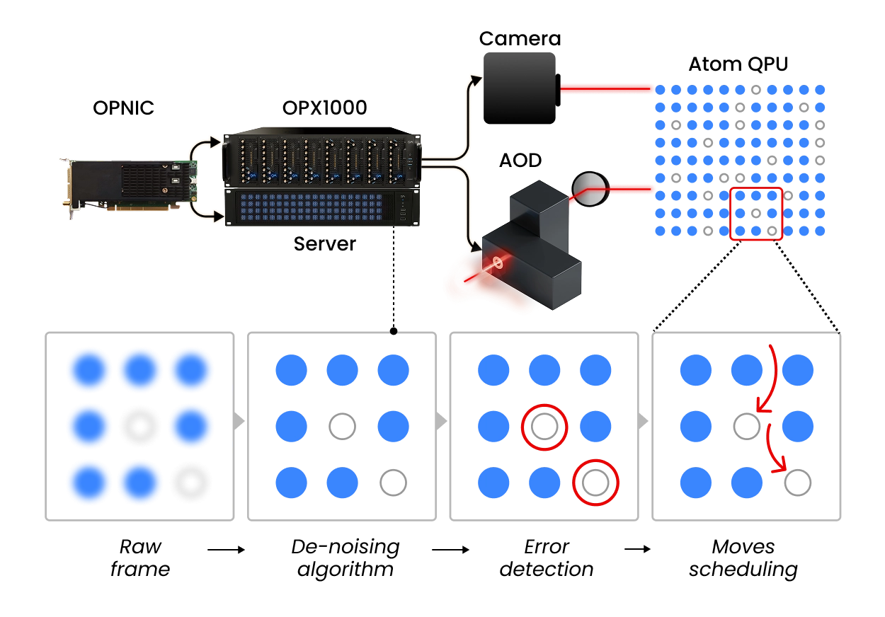
The fast-readout solution at Quantum Machines solves this with the CPU-GPU and OPX1000 interconnect using QM’s Open Acceleration Stack (OAS). OAS means that the users can connect the camera and the frame grabber to a classical accelerator which performs fast-image processing, including but not limited to using machine learning algorithms for state discrimination. The OPNIC shuttles the information back to the OPX1000. These moves can be conditional and instruct the controller to perform algorithms as needed. This also opens the possibility of using transport and routing algorithms that are more involved and are needed for scaling neutral atoms arrays.


The QUA Python interface is great, everything you want to do is just three intuitive lines of code. The OPX is one of the only things in the lab that is working exactly as it should.

Carl J. and Brynn B. Anderson Assistant Professor in Physics
Postdoctoral Fellow
The first time I was introduced to Quantum Machines, It surprised me how people were getting so excited about it. Only later did I realize, it was like explaining the value of a Laser before it existed, and all you knew are light bulbs. Today I truly believe that these systems will revolutionize our space.

Prof. Barak Dayan
Professor
The flexibility of the OPX for generating complex signals has been instrumental in our ongoing work advancing the performance of neutral atom qubit systems.

Prof. Mark Saffman
Professor
FAQ
What advantages do neutral atoms offer over ion traps?
Neutral atoms offer architectural and scaling advantages over ions. Unlike ions, neutral atoms are not charged, resulting in the absence of interactions with stray electric fields and interatomic interactions unless activated by Rydberg interaction.
Additionally, neutral atoms use optical tweezers to trap atoms within grids of easily reconfigurable geometry with interatomic spacings down to a few micrometers. In contrast, ions, which employ Paul traps, face challenges in scaling to higher-dimensional grids and accommodating a larger number of atoms. Furthermore, most ion traps exhibit a fixed linear order, rendering arbitrary connectivity, geometry, or the shuttling of qubits more intricate.
Integrated control stacks are indispensable for large-scale neutral atom arrays. Precise laser control is paramount for shuttling and applying multiple parallel two-qubit gates to establish coupling across extended distances, distinguishing them from other modalities.
What limits two-qubit gate performance in Rydberg-based systems?
High‑fidelity and low‑latency gates are essential for a quantum error correction cycle where errors are detected and then operations are applied to correct them. In neutral‑atom systems two‑qubit operations are implemented using Rydberg blockade, which requires briefly promoting atoms into extremely short‑lived, highly polarizable states to generate strong interactions. However, Rydberg gates suffer from fundamental limits like finite Rydberg lifetimes and imperfect blockade. On the control stack side, improving gate fidelity demands ultrafast, high‑power, phase‑stable laser pulses with sub‑micron pointing and nanosecond timing. These together make reaching QEC‑grade fidelity and latency challenging.
What role does atom rearrangement play?
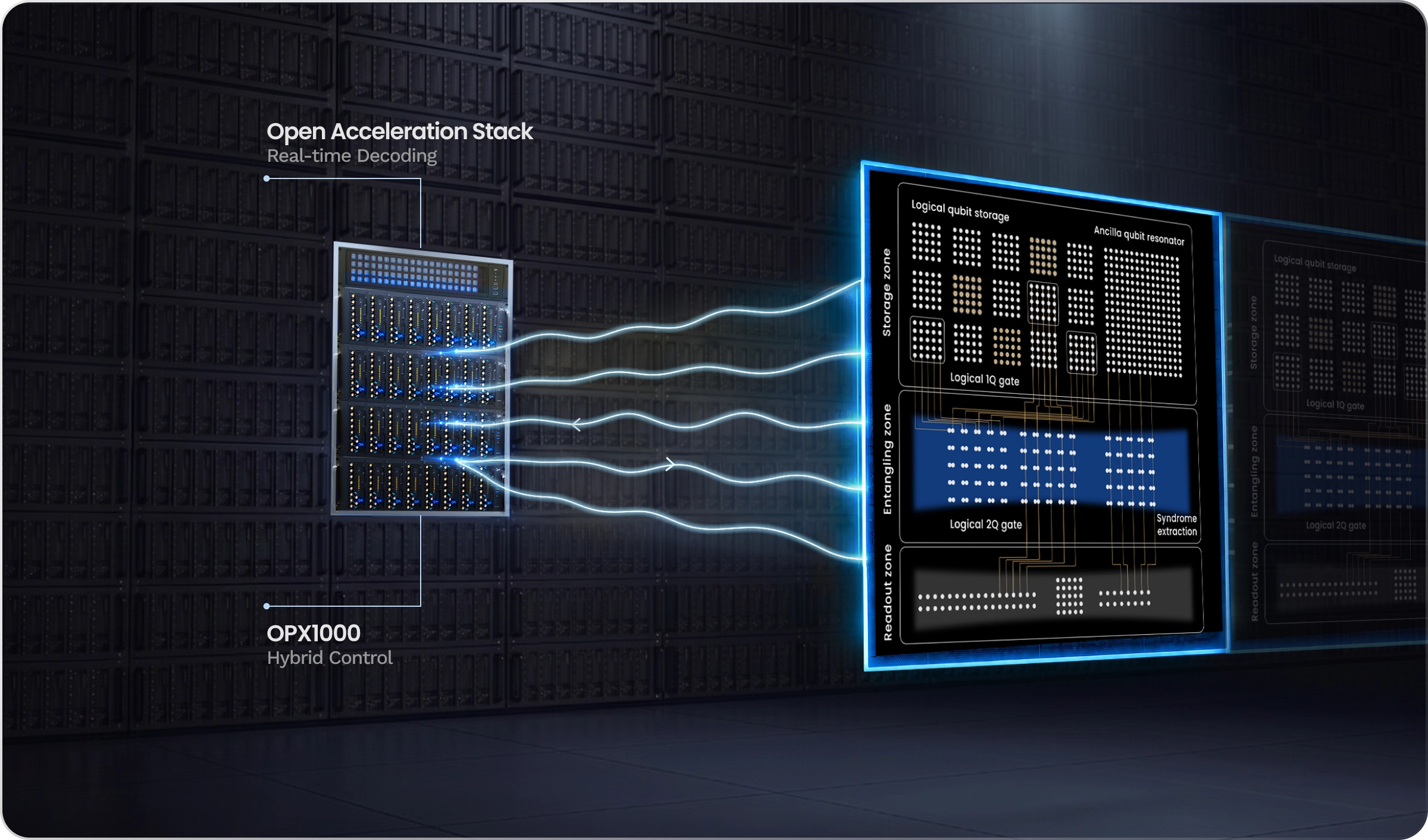
A major advantage of neutral atoms is the ability to re-position and shuttle atoms around during the experiment. This makes it possible to change the configurations of the atoms and therefore allows for all-to-all connectivity. This also enables unique capabilities, such as zone-based architectures comprising three regions: a storage zone for a reservoir of atoms, an entanglement zone for repositioning and performing interactions, and a measurement zone for readout of the atoms’ states. Atom rearrangement means that atoms can freely shuttle between the zones. Crucially supported by atom arrangement, these capabilities enable neutral atoms to apply transversal gates and execute quantum error correction algorithms.
Standard architecture uses a spatial light modulator (SLM) to create a static array of optical tweezers, and a pair of crossed AODs (2D AOD) to generate dynamic traps for atom transport. To move many atoms simultaneously and reconfigure large arrays, the OPX1000 provides multi-tone RF signals to the AOD, with each tone corresponding to a tweezer position. The Pulse level programming language QUA allows to seamlessly go from physical lab parameters like grid spacing to sophisticated rearrangement algorithms that efficient transport atoms without losing them.
Why is real-time classical processing important in neutral atom systems?
Real-time classical processing means that computation and the response to it (deciding to play and generate waveforms parametrically) happens within the coherence time of the neutral atom qubit.
For neutral atoms in particular real time is, when the readout, computations on them and generation of pulses to perform the next round of atom arrangements and gate operations can be modified mid-circuit. An example of this is in atom transport. Every OPX100 LF-FEM controlled tweezer calculates the trajectory in frequency and amplitude space while it is playing. Therefore, the latency from deciding which move to execute to the first sample out of the DAC (digital-to-analog converter) is a few microseconds. The core synthesizes waveforms on-the-fly using piecewise linear chirping in 800 nanosecond segments, calculating the next segment while playing the current one.
As neutral‑atom systems scale, they require real‑time parallel processing and adaptive control such that circuit parameters and control flow update in real-time based on mid‑circuit measurements. Modular stacks and external orchestration can’t meet the timing demands. QUA, the OPX1000’s native pulse‑level language, enables true real‑time adaptive control by running concurrent processes like atom transport and reservoir refilling based on mid-circuit readouts directly on the controller.
What becomes critical for fault tolerance in neutral atoms?
Fault-tolerant quantum computing (FTQC) entails executing computations even in the presence of errors.
The realization of FTQC necessitates the presence of three key components: logical qubits, fault tolerance, and quantum error correction (QEC). Logical qubits possess the capability to encode information across multiple physical qubits, thereby safeguarding against errors. Fault tolerance enables the suppression of errors that may arise. QEC identifies and rectifies errors within the physical qubits. As the system expands, each of these components must be optimized and executed concurrently, presenting a fundamental challenge in the realm of physics and control systems.
For neutral atoms, scaling depends on stable trapping, low‑loss transport, low‑latency readout, and precise individual control. A major challenge remains the fidelity of two‑qubit gates based on Rydberg interactions, which must improve while keeping crosstalk low. Large arrays also require careful strategies for atom motion like how far atoms move, how many move at once, and how laser‑control complexity grows with system size. Rearrangement must be fast, accurate, and loss‑free, and readout must be high‑fidelity and non‑destructive.
Distributed control stacks and external orchestration cannot meet these latency and fidelity demands. Fault tolerance ultimately demands tightly integrated, real‑time classical–quantum orchestration, with adaptive control and high parallelism to keep error rates below threshold as systems scale. These are capabilities that architectures like the OPX1000 and the QUA programming model are explicitly designed to provide.
What distinguishes an integrated quantum orchestration platform from modular instrument stacks?
The Quantum Orchestration Platform (QOP) unifies pulse generation, real‑time classical processing, control flow, and ultrafast analog feedback within a single deterministic system. Distributed control architectures split these functions across separate modules and rely on external orchestration, introducing latency and nondeterministic timing.
Within each OPX1000, the Pulse Processing Unit (PPU), an FPGA based processing unit, combines waveform generation, digitization, and real‑time computation. QUA, OPX1000’s native programming language, unifies pulse‑level control with Turing‑complete classical logic, enabling adaptive, measurement‑conditioned execution without external‑processor latency. It scales naturally from one qubit to thousands through coordinated OPX1000 controllers and a shared configuration file, with the compiler handling synchronization automatically.
This integrated quantum orchestration platform removes latency, optimizes performance, and enables real-time quantum-classical interaction. This comprehensive platform enables researchers to design, execute, and optimize quantum control protocols across diverse quantum hardware platforms.
How does control architecture impact scalability beyond 100 qubits?
As quantum computers scale up in size and utility, the performance of control systems becomes a critical factor in making the best of any quantum processing unit.
For neutral atoms, scaling depends on stable trapping, low‑loss transport, low‑latency readout, and precise individual control. A major challenge remains the fidelity of two‑qubit gates based on Rydberg interactions, which must improve while keeping crosstalk low. Large arrays also force architectural choices about how to scale: a zoned approach, where computation happens in designated regions with local rearrangement, limits how fast the laser‑control stack must grow; whereas a networked approach distributes several smaller QPUs connected optically or through fibers, shifting complexity from local control to interconnects and routing. Both approaches still require careful strategies for atom motion like how far atoms move, how many move at once, and how to keep rearrangement fast, accurate, and loss‑free along with high‑fidelity, non‑destructive readout.
Distributed control stacks and external orchestration cannot meet these latency and fidelity demands. Fault tolerance ultimately demands tightly integrated, real‑time classical–quantum orchestration, with adaptive control and high parallelism to keep error rates below threshold as systems scale. These are the capabilities that architectures like the OPX1000 and the QUA programming model are explicitly designed to provide.
Why is embedded real-time classical processing important for neutral atom systems?
Real-time classical processing means that computation and the response to it (deciding to play and generate waveforms parametrically) happens within the coherence time of the neutral atom qubit.
Within each OPX1000, the Pulse Processing Unit (PPU), an FPGA based processing unit, combines waveform generation, digitization, and real‑time computation. QUA, OPX1000’s native programming language, unifies pulse‑level control with Turing‑complete classical logic, enabling adaptive, measurement‑conditioned execution without external‑processor latency. This means that compute, control and create waveforms happen in the same system simultaneously without the need of external system for decision logic. This allows for real-time control flow e.g. if/else, switch cases etc statements to condition operations in real time.
How does architecture choice impact long-term roadmap viability?
The architecture of a quantum control stack determines its scalability. A Quantum Orchestration Platform (QOP) integrates pulse generation, real-time classical processing, control flow, and ultrafast analog feedback into a single deterministic system. In contrast, distributed control architectures separate these functions across modules and depend on external orchestration, introducing latency, timing uncertainty, and coordination overhead that compound as the system grows.
Each OPX1000 has a FPGA-based Pulse Processing Unit (PPU) that tightly combines waveform generation, digitization, and real-time computation. QUA, the OPX1000’s native programming language, unifies pulse-level control with Turing-complete classical logic, enabling fully adaptive, measurement-conditioned execution without external processor latency. It scales from a few qubits to thousands through coordinated OPX1000 controllers and a shared configuration file, with the compiler automatically handling synchronization, timing, and data exchange.
QUA programs don’t need rewriting as the system expands, so scaling becomes adding controllers and updating configuration, not re-architecting control logic. This deterministic, tightly integrated approach provides a clear path to long-term scalability, unlike distributed stacks with inherent latency and synchronization constraints.
Scale
Fault-tolerant neutral-atom computation demands a control system that operates natively at the gate physics timescale: real-time pulse shaping, dynamic frequency adaptation, chirp correction, feed-forward from mid-circuit measurement outcomes, and adaptive atom transport. All resolved within microseconds, continuously, across weeks of autonomous operation. That requires more than a waveform uploader that streams precompiled pulses.
Quantum Machines’ hybrid control stack is built for this architecture. QM’s OPX1000 and Open Acceleration Stack can deliver nanosecond-precision pulse control, real-time QEC decoding, mid-circuit readout processing, and adaptive AOD control, all under a single hardware-abstracted software layer.
The result is an end-to-end platform covering installation, system integration, calibration, and dedicated physics and engineering support from day one. This means that from the first photon to fault-tolerant logical qubit, every layer is covered, so your team can focus on the algorithms rather than the infrastructure.
Set Up Architecture
Quantum-Classical Integration and Control Highlights
A control stack for mid-circuit calibrations
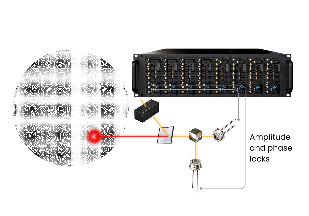
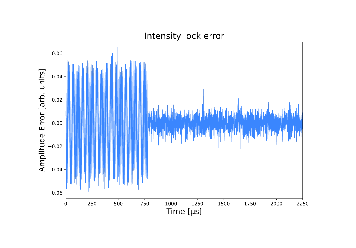
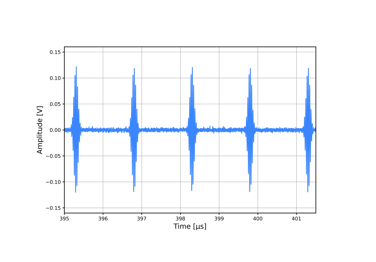
Laser frequencies in a neutral atoms’ setup can drift in microseconds timescale directly impacting the fidelity of the gates, transport and control. Treating calibration as an offline step means that the QPU you started with is not the one you are running your circuit on. Without continuous calibration, running jobs for hours is impossible.
An integrated control system can overcome this. Atom transport intervals between gate zones can be free calibration windows. With OPX1000 on-the-fly pulse generation and microsecond feedback from a CPU/GPU server offered by the Open Acceleration Stack, laser parameters can be continuously monitored, updating pulse amplitudes, phases, and frequencies at slice synchronization points so corrections remain coherent and never interrupt the running program. Closed loop frequency and intensity stabilization can run on QUA persistently alongside computation. Furthermore, mid-circuit readout can feed site-resolved phase corrections back into the next gate slice within the same job.
The OPX1000 and Open Acceleration Stack, with OPNIC bridging low-latency GPU acceleration into the control loop, provide the substrate for exactly this architecture. On-the-fly pulse shaping and real-time chirp control, deterministic AOD drive sequencing, and a unified classical stack where calibration logic and gate execution share the same real-time layer is imperative for fault-tolerant operation.
Gate Addressing at Scale
Driving individual gates on thousands of atoms simultaneously pushes optics past its limits. In practice, parallelism and phase uniformity degrade, and reconfiguring beam paths per experiment becomes costly for a production-level QPU system.
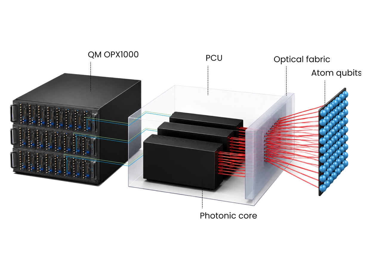
Mach-Zehnder interferometer-based photonic integrated chips (PIC) offer a scalable solution to this challenge. Hundreds of individually addressable channels can be routed, phased, and intensity-controlled on a centimeter-scale chip fabricated via standard semiconductor processes. This replaces free-space optics with a stable, reconfigurable integrated architecture. Swappable photonic cores keep the platform forward compatible as qubit arrays grow.
QM’s OPX1000 provides the high-speed analog signal generation, real-time pulse programming, and hardware-abstracted software layer that drives these photonic chips from physical signal to gate-level instruction. The same platform that closes the calibration loop at the microsecond timescale now extends that real-time control all the way to the photonic layer.
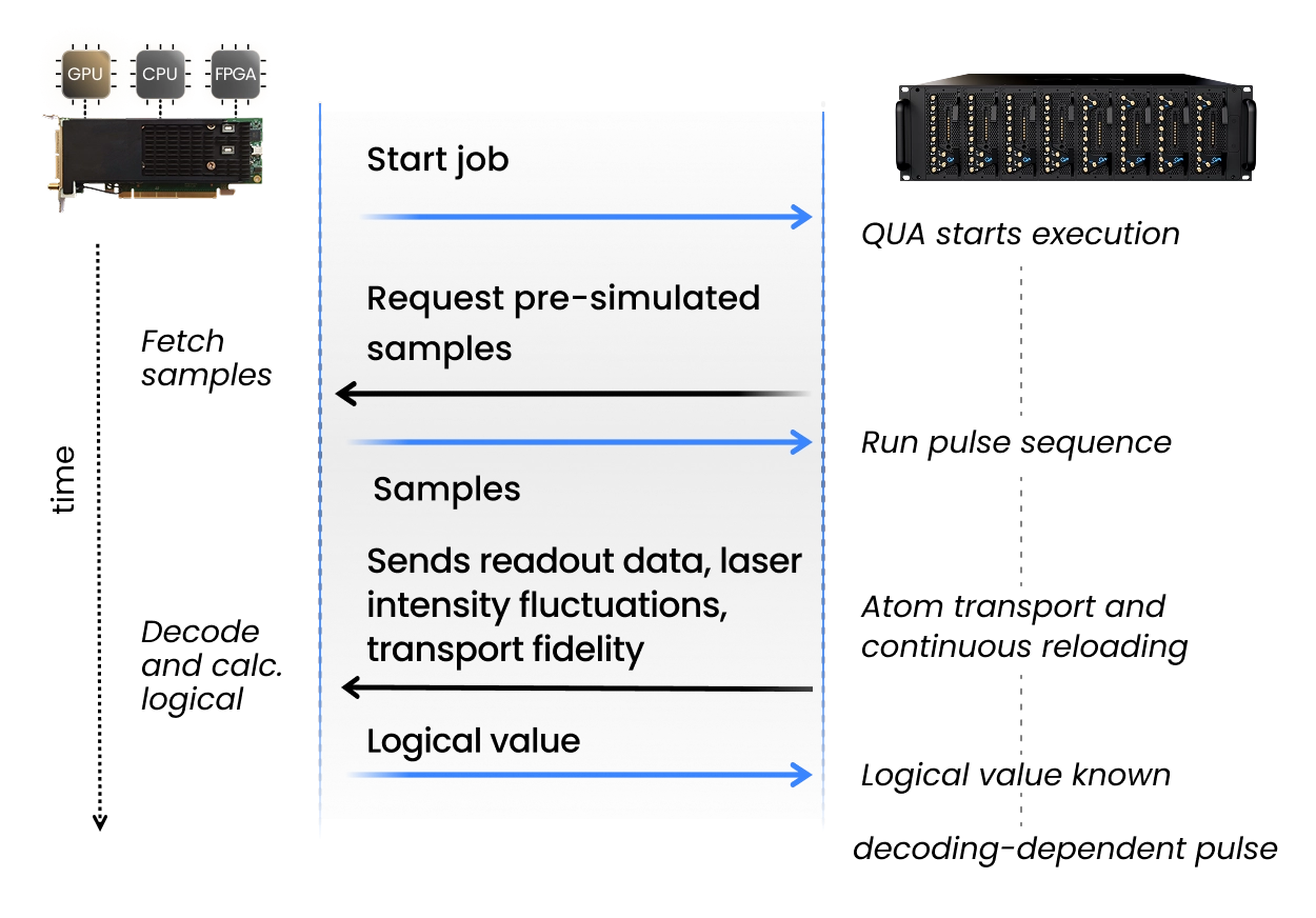
Real-time decoding and feedforward
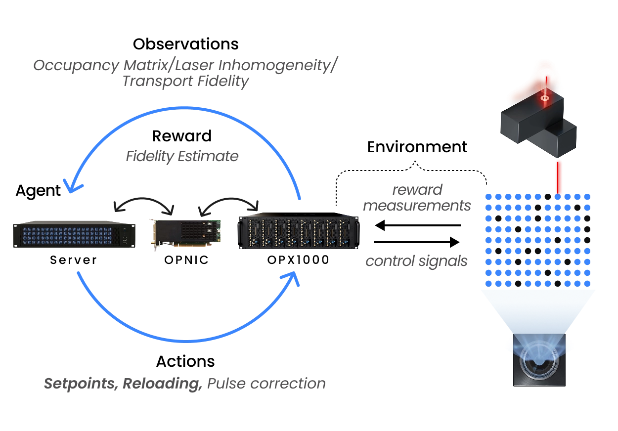
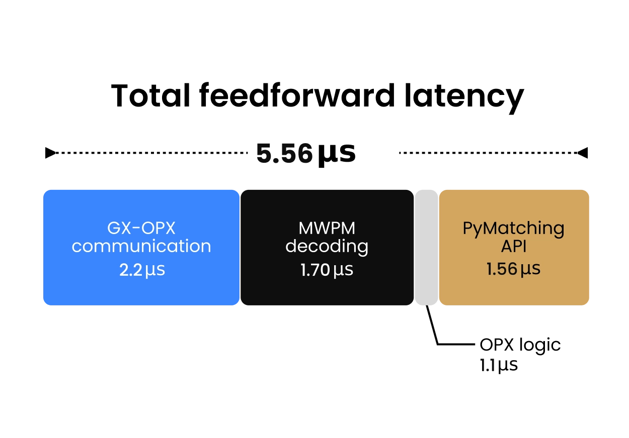
Fault-tolerant operation requires every classical decoding, branching, and feed-forward to close its loop before the next QEC cycle begins. QM’s OPX1000 generates syndromes, and our Open Acceleration Stack delivers them to a CPU/GPU server, where logical control flow lives. Branching decisions are made classically on the server and returned to the QPU as the next instruction.
This works because decoding is faster than transport. QM’s OPNIC closes the QPU-to-server roundtrip in under 2-4 µs, meaning the decoded result arrives back at the control layer faster than an atom can be shuttled across a zone boundary. OPNIC slots into the server as a standard PCIe card, making the quantum controller a native backplane device and eliminating network latency entirely. The server becomes a genuine real-time agent inside the loop rather than a post-processing observer.
Syndrome routing happens dynamically. Straightforward cases are resolved locally in the OPX1000, while harder syndromes are dispatched over the OPNIC to the server decoder and the result applied immediately as the next pulse. Quantum control, decoding, and classical orchestration operate as one closed-loop system.
The QUA Python interface is great, everything you want to do is just three intuitive lines of code. The OPX is one of the only things in the lab that is working exactly as it should.
Carl J. and Brynn B. Anderson Assistant Professor in Physics
Postdoctoral Fellow
The first time I was introduced to Quantum Machines, It surprised me how people were getting so excited about it. Only later did I realize, it was like explaining the value of a Laser before it existed, and all you knew are light bulbs. Today I truly believe that these systems will revolutionize our space.
Prof. Barak Dayan
Professor
The flexibility of the OPX for generating complex signals has been instrumental in our ongoing work advancing the performance of neutral atom qubit systems.
Prof. Mark Saffman
Professor

Blog
Turning Latency into an Advantage: Continuous Calibration for Neutral-Atom Quantum Computers
Read more June 2026 | 8 min read
Blog
Classically Accelerated Readout for Neutral Atoms with CPU/GPU Integration
Read more June 2026 | 8 min read
Scientific Publications
Loss Mechanisms in High-coherence Multimode Mechanical Resonators Coupled to Superconducting Circuits
Read more May 2026 | 1 min read
Scientific Publications
Learning Nonlinear Heterogeneity in Physical Kolmogorov-Arnold Networks
Read more May 2026 | 1 min readFAQs
What distinguishes an integrated quantum orchestration platform from modular instrument stacks?
The Quantum Orchestration Platform (QOP) unifies pulse generation, real‑time classical processing, control flow, and ultrafast analog feedback within a single deterministic system. Distributed control architectures split these functions across separate modules and rely on external orchestration, introducing latency and nondeterministic timing.
Within each OPX1000, the Pulse Processing Unit (PPU), an FPGA based processing unit, combines waveform generation, digitization, and real‑time computation. QUA, OPX1000’s native programming language, unifies pulse‑level control with Turing‑complete classical logic, enabling adaptive, measurement‑conditioned execution without external‑processor latency. It scales naturally from one qubit to thousands through coordinated OPX1000 controllers and a shared configuration file, with the compiler handling synchronization automatically.
This integrated quantum orchestration platform removes latency, optimizes performance, and enables real-time quantum-classical interaction. This comprehensive platform enables researchers to design, execute, and optimize quantum control protocols across diverse quantum hardware platforms.
How does control architecture impact scalability beyond 100 qubits?
As quantum computers scale up in size and utility, the performance of control systems becomes a critical factor in making the best of any quantum processing unit.
For neutral atoms, scaling depends on stable trapping, low‑loss transport, low‑latency readout, and precise individual control. A major challenge remains the fidelity of two‑qubit gates based on Rydberg interactions, which must improve while keeping crosstalk low. Large arrays also force architectural choices about how to scale: a zoned approach, where computation happens in designated regions with local rearrangement, limits how fast the laser‑control stack must grow; whereas a networked approach distributes several smaller QPUs connected optically or through fibers, shifting complexity from local control to interconnects and routing. Both approaches still require careful strategies for atom motion like how far atoms move, how many move at once, and how to keep rearrangement fast, accurate, and loss‑free along with high‑fidelity, non‑destructive readout.
Distributed control stacks and external orchestration cannot meet these latency and fidelity demands. Fault tolerance ultimately demands tightly integrated, real‑time classical–quantum orchestration, with adaptive control and high parallelism to keep error rates below threshold as systems scale. These are the capabilities that architectures like the OPX1000 and the QUA programming model are explicitly designed to provide.
Why is embedded real-time classical processing important for neutral atom systems?
Real-time classical processing means that computation and the response to it (deciding to play and generate waveforms parametrically) happens within the coherence time of the neutral atom qubit.
Within each OPX1000, the Pulse Processing Unit (PPU), an FPGA based processing unit, combines waveform generation, digitization, and real‑time computation. QUA, OPX1000’s native programming language, unifies pulse‑level control with Turing‑complete classical logic, enabling adaptive, measurement‑conditioned execution without external‑processor latency. This means that compute, control and create waveforms happen in the same system simultaneously without the need of external system for decision logic. This allows for real-time control flow e.g. if/else, switch cases etc statements to condition operations in real time.
How does architecture choice impact long-term roadmap viability?
The architecture of a quantum control stack determines its scalability. A Quantum Orchestration Platform (QOP) integrates pulse generation, real-time classical processing, control flow, and ultrafast analog feedback into a single deterministic system. In contrast, distributed control architectures separate these functions across modules and depend on external orchestration, introducing latency, timing uncertainty, and coordination overhead that compound as the system grows.
Each OPX1000 has a FPGA-based Pulse Processing Unit (PPU) that tightly combines waveform generation, digitization, and real-time computation. QUA, the OPX1000’s native programming language, unifies pulse-level control with Turing-complete classical logic, enabling fully adaptive, measurement-conditioned execution without external processor latency. It scales from a few qubits to thousands through coordinated OPX1000 controllers and a shared configuration file, with the compiler automatically handling synchronization, timing, and data exchange.
QUA programs don’t need rewriting as the system expands, so scaling becomes adding controllers and updating configuration, not re-architecting control logic. This deterministic, tightly integrated approach provides a clear path to long-term scalability, unlike distributed stacks with inherent latency and synchronization constraints.