QM’s Orchestration Platform for
Quantum Networks
Orchestrate spin-photon interfaces, remote-node protocols, and heralded entanglement with synchronized optical, microwave, RF, and photon-detection control. QM’s Orchestration Platform enables real-time branching, repeat-until-success workflows, and phase-coherent memory control for scalable quantum networking experiments.


QUANTUM NETWORKS
Research
Quantum networks aim to distribute high-quality entanglement between remote quantum nodes, enabling new approaches to quantum communication, photonic computing, metrology, and distributed quantum processing. These protocols often rely on spin-photon interfaces, memory qubits, photon detection, and local operations that must work together while errors, loss, and decoherence are kept under control. Platforms such as Defect Centers are especially powerful for these experiments, combining optically addressable communication qubits with nearby nuclear-spin memories, but many platforms promise quantum networks operations, from heterostructure quantum dots to ion-based single photon sources.
Quantum Machines’ Orchestration Platform supports quantum-network experiments by synchronizing optical pulses, microwave and RF control, photon time tagging, memory operations, and real-time decision-making from one platform. Powered by OPX hybrid controllers and the Pulse Processing Unit, QM enables heralded entanglement, repeat-until-success loops, node synchronization, phase tracking, and distillation protocols that react immediately to measurement outcomes. With QUA, complex network sequences can be written as intuitive, reusable workflows, helping researchers move faster from individual node control to scalable quantum-network protocols.
Spin-Photon Interfaces for Remote Entanglement
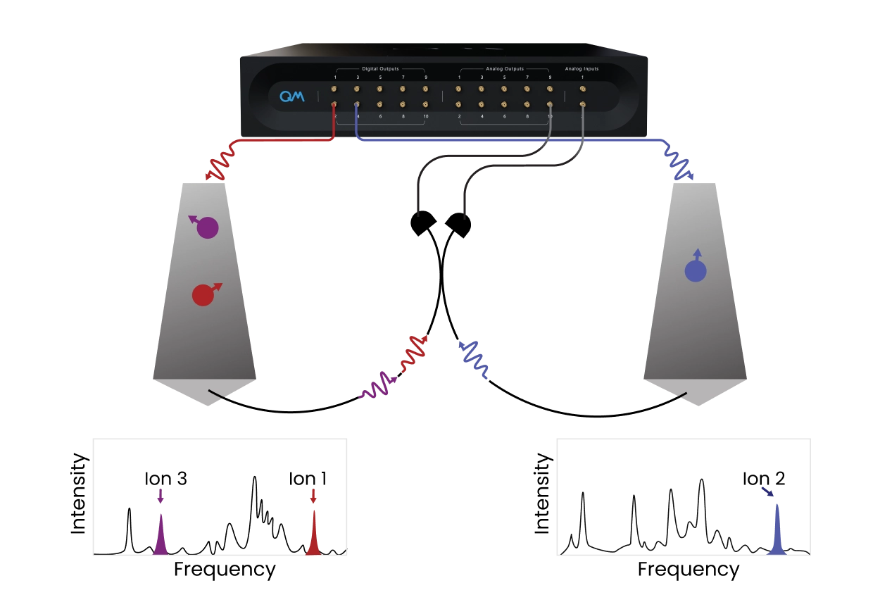
Quantum networks rely on photons to generate entanglement between remote quantum nodes while local memory qubits preserve quantum information. Experiments such as scalable multipartite entanglement of remote rare-earth ion qubits show the promise of optically addressable systems for distributed quantum architectures [e.g. Ruskuc, A., Nature 639, 54–59 (2025)]. QM’s Orchestration Platform synchronizes optical excitation, microwave/RF control, photon collection, time tagging, and conditional local operations in one workflow. With OPX and QUA, researchers can program spin-photon protocols at the pulse level, process detection events in real time, and move from single-node control to remote entanglement experiments.
Repeat-Until-Success for non-Deterministic Sequences Across Quantum Nodes
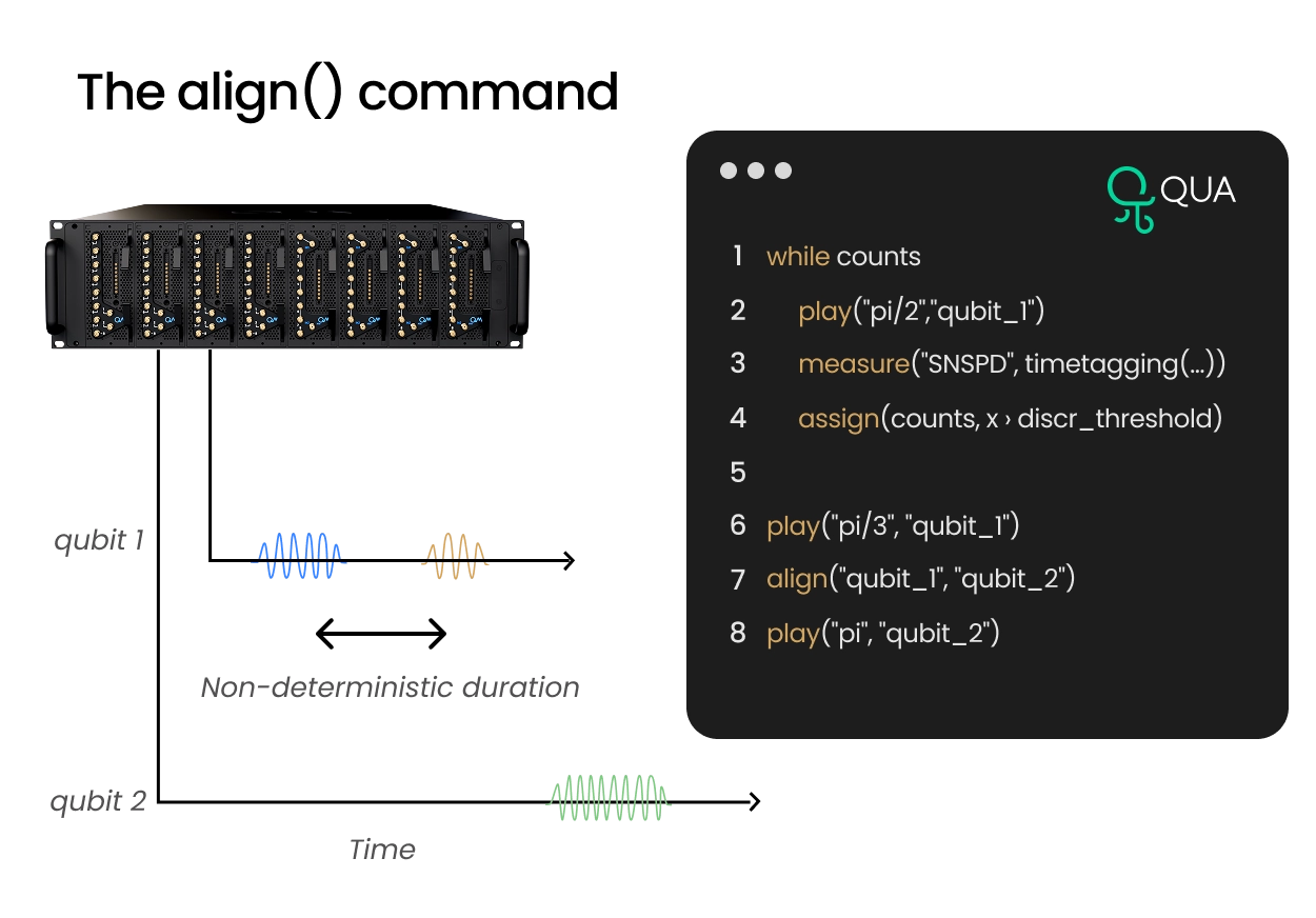
Quantum-network protocols are often non-deterministic: one node may succeed after a single attempt, while another may require many repetitions before a heralding event occurs. This makes fixed timing and static sequencing inefficient. Thanks to the intuitive align() command, QM’s Orchestration Platform enables repeat-until-success workflows directly on the controller. OPX can run independent node sequences in parallel, process photon counts and time tags in real time, evaluate success conditions, and align nodes only when each has reached the required checkpoint. With QUA, loops, counters, conditionals, and synchronization commands are written intuitively, allowing complex heralded protocols to run without slow software intervention or fragmented external logic.
Entanglement Distillation with Phase-Coherent Control
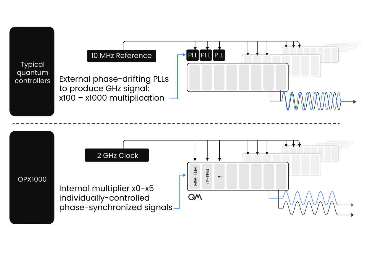
Entanglement distillation depends on more than real-time logic. To turn multiple imperfect entangled states into fewer, higher-fidelity ones, the controller must preserve phase coherence across repeated attempts, local gates, memory operations, and measurement-based decisions. Any timing jitter or phase noise can reduce the fidelity of the distilled state. QM’s Direct Digital Synthesis architecture provides a fundamentally more stable control layer by generating microwave signals directly from digital data, with deterministic phase control, low phase noise, and a shared high-frequency clocking architecture. Compared with customary 10 MHz-referenced instrument chains, the OPX1000’s 2 GHz timing foundation helps maintain phase stability across long, repeated, and branching network protocols.

The Quantum Machines OPX control system has been an enabling technology for our research. It provides unparalleled flexibility and ease of use for experiments requiring real-time quantum feedforward control. With the integrated high-resolution time tagging, this platform is a no-brainer for advanced quantum networking experiments.

Prof. Andrei Faraon
Optical and Quantum Engineer

Blog
Blog
Pioneering Quantum Networking: Achieving Scalable Entanglement of Remote Distinguishable Qubits
Read more March 2025 | 6 min read
Blog
European Institutions Announce Research Project to Develop Neural Networks for Quantum Error Correction
Read more April 2022 | 3 min read
Blog
Machine Learning for Quantum Processing: How to Run Real-Time Neural Networks
Read more June 2021 | 4 min readFAQ
What is heralded entanglement, and how does the platform react to heralding events in real time?
Heralded entanglement uses a detected photon to confirm that a remote-entanglement attempt succeeded, so the protocol only advances on verified successes rather than assuming every attempt worked. The OPX takes single-photon detector signals directly and processes photon counts and time tags natively, letting the controller evaluate the heralding condition and branch (continue, store to memory, or retry) within the same synchronized sequence. Keeping that decision on the controller avoids the latency of routing detection data out to external software.
How does the platform run non-deterministic, repeat-until-success network protocols?
Network protocols are inherently non-deterministic. One node may succeed on the first attempt while another needs many tries before a heralding event. So the OPX handles the branching on the controller rather than in slow external logic. It runs independent node sequences in parallel, evaluates success conditions from real-time photon data, and repeats attempts until each node reaches its checkpoint. In QUA, the loops, counters, conditionals, and synchronization commands (such as align()) these workflows need are written intuitively as reusable code.
How does the OPX keep multiple remote nodes synchronized?
The OPX runs each node’s sequence independently and in parallel, then aligns them only once each has reached its required checkpoint. This means that faster nodes wait for slower ones instead of forcing inefficient fixed timing. This matters precisely because, as QM notes, you cannot predict in advance how long each node will take to reach a checkpoint. Real-time evaluation of each node’s state on the controller is what keeps the protocol coordinated despite that unpredictability.
How does Quantum Machines preserve phase coherence for entanglement distillation and long protocols?
Distillation is converting several imperfect entangled pairs into fewer, higher-fidelity ones. It depends on preserving phase coherence across repeated attempts, local gates, memory operations, and measurement-based decisions, since any timing jitter or phase noise degrades the distilled state. QM’s Direct Digital Synthesis architecture provides a more stable control layer by generating microwave signals directly from digital data, with deterministic phase control, low phase noise, and a shared high-frequency clock. The OPX1000’s timing foundation helps hold phase stability across long, repeated, and branching network protocols, which also benefits quantum sensing.
Which qubit platforms are suited to quantum networks, and does QM support them?
Optically addressable platforms are especially powerful here, pairing a communication qubit that emits photons with a nearby memory qubit. Defect centers are a leading example, combined with nuclear-spin memories, alongside rare-earth ions, heterostructure quantum dots, and ion-based single-photon sources. QM’s platform drives these spin-photon systems from a single controller, coordinating the optical, microwave, RF, and photon-detection channels each one requires. That same flexibility is why the platform spans defect-center computing, sensing, and networking without rebuilding the control stack.
Why aren’t traditional instruments well suited to quantum-network experiments?
Traditional setups struggle because network protocols are dominated by repeat-until-success blocks with unpredictable timing, which static, pre-defined sequences handle inefficiently. As QM puts it, using traditional equipment is challenging because of the abundance of repeat-until-success blocks, especially since you cannot predict in advance how long each node will take to reach a checkpoint. The OPX replaces fragmented external logic with on-controller real-time decision-making, so heralded protocols run without slow software round-trips.