Quantum Control for
Defect Centers & Optically Addressable Qubits

The OPX line of quantum controllers (OPX+ and OPX1000) offers exceptional capabilities for all qubits that are optically addressable or those with photon-based readouts, such as NV centers, other defect centers and most other quantum photonics platform. Specifically, it contains all your control needs integrated in one box. This includes photon counters and time taggers; microwave (MW) and radio-frequency (RF) pulse generators; external device controllers, such as modulators – AOMs, EOMs & AODs, piezo stages, strain tuners, MEMs devices, etc.; digital triggers; classical resources to analyze, compute and modify the control in real-time. OPX is the orchestration device you need for all your experiments in the Quantum Photonics space. This includes neutral atoms and ions, for which we direct the reader onto the specific page.

OPX is an all-in-one solution to control optically active spins in many material platforms including diamond, silicon-carbide, silicon, hBN, and oxydes whether they are intrinsic (e.g. NV center) or substitutional (e.g. rare earth elements) in nature. OPX is the ideal tool for the optically active spin defects community from materials science research to quantum computing. Our proprietary Pulse Processing Unit (PPU) powers the OPX, offering many functionalities, from basic qubit characterization to multi-NMR control sequences, all easily and intuitively implemented in a single box. OPX not only can increase throughput by rapid qubit characterization but can also implement  time-synchronized non-deterministic sequences such as heralding schemes for quantum networks, transduction, quantum sensing, quantum photonics and computing. The OPX capabilities and the all-to-all connectivity between its cores and outputs allow for maximum flexibility and productivity.

The OPX’s instruction-based system allows one to easily code any experiment (check out our blog for a fresh POV of an experimentalist). The user writes high-level commands in QUA, our python-embedded pulse-level programming language. Then, the PPU compiles and executes these coded instructions in real-time, running with virtually no compilation time or memory overhead for arbitrarily long sequences (yes, this means unlimited playtime after <1 second of compilation).

Octave, an up-conversion module for the OPX, offers seamless operation up to 18 GHz with auto-calibrated mixers, for a fully plug-and-forget solution. At the same time, the OPX1000, Quantum Machines’ large-scale quantum controller offers a solution without calibration up to 10.5 GHz, thanks to direct digital synthesis.

Let’s see some examples, from basic to more advanced.

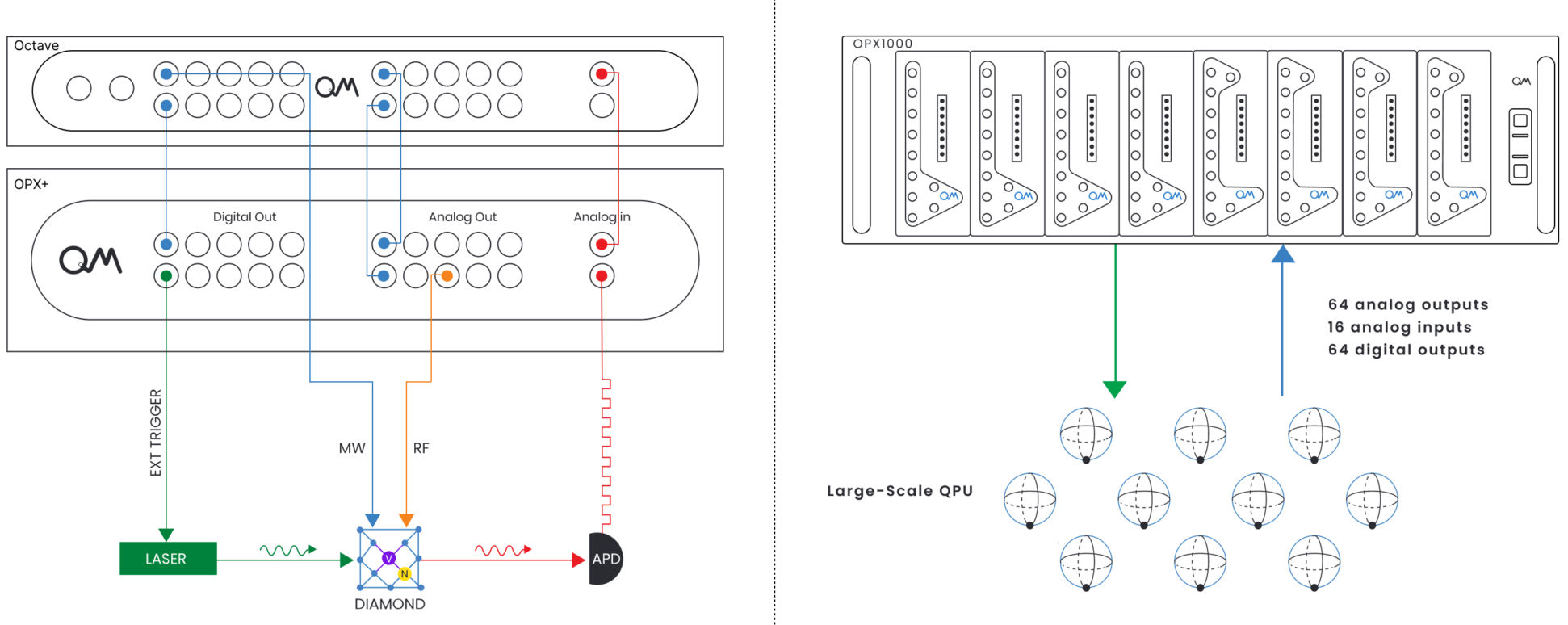
Fig. 1. (Left) Standard OPX+ setup used for radio-frequency (RF) and microwave (MW) combined control on NV centers in diamond. The OPX+ orchestrates the experiment and triggers lasers that drive the qubits. RF (DC-400MHz) is provided directly from the OPX, while the Octave addon offers MW up-conversion with automated calibration for a plug-and-forget system. The OPX time-tags the detector output for analysis, computation, and feedback. One OPX analog input can be used to automatically calibrated the Octave mixers, or alternatively to time-tag more than one detector, allowing for e.g. correlation experiments. OPX can orchestrate many devices using both analog signals and digital triggers, making it truly an all-in-one solution for quantum photonics. (Right) The same features and orchestrating options are available for the large-scale quantum controller, the OPX1000, with separate modules for RF and MW, working up to 10.5 GHz without mixers and without calibration, ensuring the best of performances at scale.

As an illustrative example, we show a standard NV center experimental setup in Figure 1. We can easily convert this design for any other optically addressable qubit, with additional output channels triggering other instruments or driving various devices such as Stark pads, MEMS structures, or EOMs. All features and example below are valid for the OPX+ controlling small scale QPUs, and for the OPX1000, offering DC to 10.5 GHz operation up to thousands of channels.

Instruction-based qubit characterization

The first step is locating the spin transition frequencies to drive the qubit with a resonance experiment. For Defect Centers, such as the NV center qubit in Fig. 1, this is usually done by driving a microwave (MW) tone and a spin initialization/readout laser at the same time. The frequency of the MW is swept until a change in the emission spectrum is observed, denoting the spin transitions of interest.

To start, we define a measurement macro in QUA. With the measure() command, we analyze the incoming signal from a photon counting module (e.g. SNSPD, APD, PMT) into the ADCs as a time-tagging measurement and save both the photon arrival times in an array called times, and the number of photons as counts. These are real-time variables that live within the Pulse Processing Unit (PPU) and can be accessed throughout the execution of the program. 

# Time Tagging QUA Macro 
# provides counts and times of arrival for tags within measurement window
def get_photons():
    times = declare(int, size=100)
    counts = declare(int)
    measure("measure", "SPCM", None, time_tagging.analog(times, measurement_time, counts))
    return times, counts
times, counts = get_photons()

Then, an optically detected magnetic resonance would be implemented like the following way:

# Optically detected magnetic resonance (ODMR) QUA code 
def ODMR(f_start, f_end, f_steps):
    f = declare(int)
    with for_(f, f_start, f<f_end, f+f_steps):
        update_frequency("Qubit", f)
        align()
        play("cw", "Qubit")
        play("laser_ON","Laser")        
        times, counts = get_photons()

The for loop is implemented within the PPU and sweeps over the real-time variable with the provided parameters. play() commands generate a real-time predefined waveform (e.g., “cw”) envelope with the carrier frequency f that is parametrically changed with the for loop to look for the spin resonance. The signal is outputted from predetermined channels according to the rules defined for the “Qubit” element. Finally, the results are measured with the macro get_photons() defined earlier. Such an experiment is easily implemented with six lines of code that can be followed and understood easily. As the OPX platform is an instruction based system, there is not a difference between sweeping over 10 values or 10,000 – the system memory and the compilation overhead will be the same, saving a significant amount of time between each experiment and enabling ultra-long experiments easily.

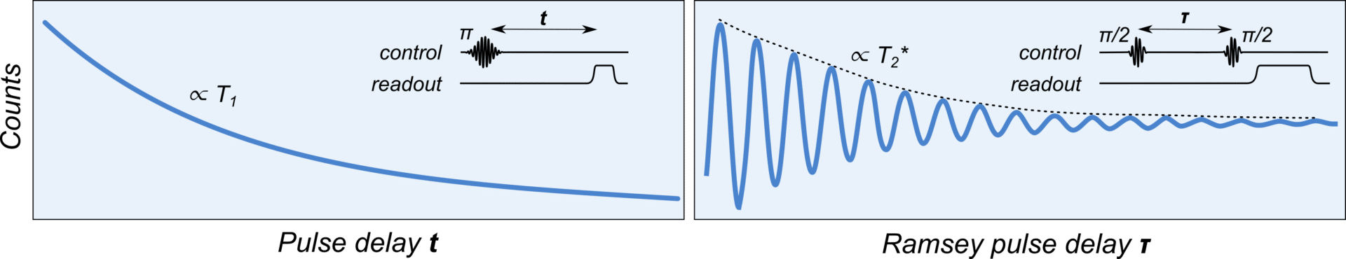
Now we continue with some examples from standard characterization experiments. Whether you use your NV center qubits (or any other) for quantum communication, computation, sensing, or other quantum photonics application, it is likely that you will need to measure coherence times and perform basic characterization, for example \(T_1\) and Ramsey experiments (see Figure 2).

Fig. 2. Sketch depicting the result of \(T_1\) and Ramsey (\(T_2^*\)) experiments, with the pulse protocols in incept.

We can compose a \(T_1\) experiment very easily by initializing the spin of our NV center qubit (Fig. 1) optically with a laser, putting it into the opposite spin state with a 𝝅-pulse and waiting to see how long it takes for it to decay back into the initialized state as a function of the geometrically increasing wait time 𝝉. The averaging loop can be placed over the entire sequence to improve the \(1/f\) noise as the system can update sweeping parameters in real-time and record its result.

# T1 protocol QUA code
def T1(N, t_start, t_end, t_mult):
    tau     = declare(int)  # time to vary
    avg_idx = declare(int)  # averaging index
    play("laser_ON", "Laser")
    with for_(avg_idx, 0, avg_idx<N, avg_idx+1):
        with for_(tau, t_start, tau<t_end, tau*t_mult):
            play("pi", "Qubit")
            wait(tau, "Qubit")
            align()
            play("laser_ON", "Laser")
            times, counts = get_photons()

Note how easy it would be to turn this code into a contrast measurement, with and without a 𝝅-pulse, and saving the respective results into a new QUA variable to calculate real-time contrast with a couple more lines of code.

Here we see an instance of the align() command, which instructs the pulse processor to wait for all channels to be done with their respective subroutines before moving to the next set of instructions. The temporal alignment of sequences works for both time-deterministic and non-deterministic sequences (e.g., heralding and other quantum photonics schemes). 

A Rabi experiment, used to calibrate control pulses, can be very easily coded similar to the \(T_1\) example, by stretching the pulse duration in real-time within the play() command, so instead of varying 𝝉  we would vary the pulse duration t:

# additional QUA code for Rabi protocol 
…
with for_(t, t_start, t<t_end, t+t_steps):
     play("cw", "Qubit", duration=t)
…

A Ramsey experiment is defined as follows: 𝝅/2-pulse, wait a variable time 𝝉, 𝝅/2-pulse again, then measure. In our experiment we can simply loop over this block by changing 𝝉  depending on the experimental needs and recording the measured counts. After averaging, we can uncover the qubits \(T_2^*\) from the decay spectrum and further calibrate the qubit’s frequency from the oscillations (this sequence is often used to build frequency-tracking ultra-fast mid-circuit calibration routines, i.e. embedded calibrations).

# Ramsey protocol QUA code to measure qubit T2*
def Ramsey(N, tau_start, tau_end, tau_steps):
   tau    = declare(int) # time to vary
   avg_idx  = declare(int) # averaging index
   play("laser_ON", "Laser")
       with for_(avg_idx, 0, avg_idx<N, avg_idx+1):
       with for_(tau, tau_start, tau<tau_end, tau+tau_steps):
            play("pi_half", "Qubit")
            wait(tau) 
            play("pi_half", "Qubit")
            align()
            play("laser_ON", "Laser")
            times, counts = get_photons()

All other characterization and calibration protocols, from echo measurements to randomized benchmarking with depth >10,000, are easy to code in QUA and run with minimal overhead – orders of magnitude faster than standard AWGs – and with the highest performance on the OPX products.

Qubit readout and time-resolved measurements

Thanks to the OPX’s wide range of functionalities, many quantum photonics, spintronics, and optics standard experiments can be performed with ease and right out of the box. This includes qubit readout, time-resolved counting measurements (TCSPC), correlation and lifetime, randomized benchmarking, and more. 

The OPX’s input channels allow event tagging with <50 ps resolution, integration, demodulation and a wide range of pre-processing and analysis on the fly. Each shot is uniquely tagged with its control, improving \(1/f\) noise and eliminating duty cycle corrections. The information from each tag can also be used right away in any feedback or feedforward protocol.

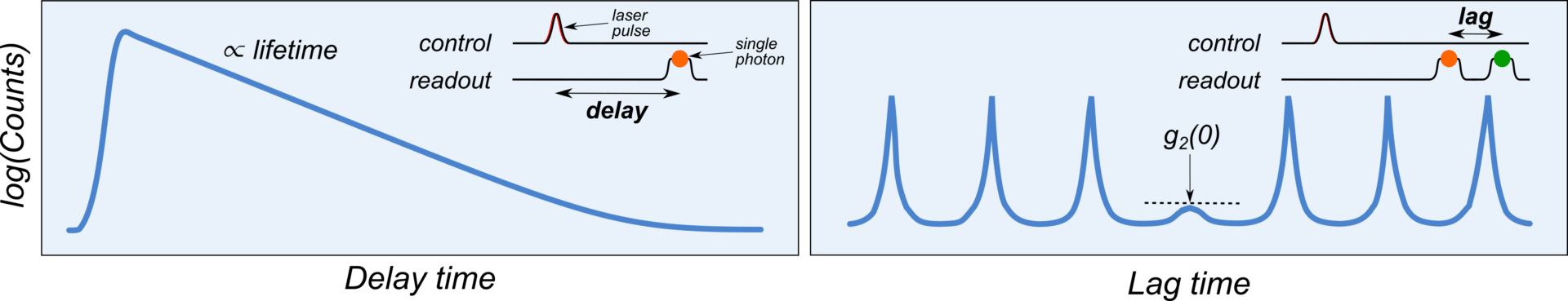
Let us take as an example a standard single-photon readout for tagging measurements such as lifetime and \(g_2\), as shown in Figure 3.

Fig. 3.Sketch depicting the result of optical lifetime and correlation (\(g_2\)) experiments, with the pulse protocols in incept.

We already saw how a tagging measurement looks in QUA (in previous tabs) and we made a get_photons() macro. Now we can use it to program optical lifetimes and correlations in just a few lines of QUA code:

# Optical lifetime measurement QUA code
def optical_lifetime(N):
     with infinite_loop():
          play("laser_ON", "laser")
          align()
          times, counts = get_photons()

# g2 correlation experiment QUA code
# able to correlate tags directly from APDs, SNSPDs, etc.
def g2_MZI(correlation_window):
    g2_vector = declare(int, size = correlation_window)
    j = declare(int)
    k = declare(int)
    difference = declare(int)
    difference_ind = declare(int)
    lower_index_tracker = declare(int)

    play("laser_ON", "Laser")
    times1, counts1 = get_photons("SPCM1")
    times2, counts2 = get_photons("SPCM2")

    assign(lower_index_tracker, 0)
    with for_(k, 0, k <= counts1, k + 1):
        with for_(j, lower_index_tracker, j <= counts2, j + 1):
            assign(difference, times2[j] - times1[k])
            with if_(difference > correlation_window):
                assign(j, counts2 + 1)
            with elif_((difference < correlation_window) & (difference > -correlation_window)):
                assign(difference_ind, difference + correlation_window)
                assign(g2_vector[difference_ind], g2_vector[difference_ind] + 1)
            with elif_(difference < -correlation_window):
                assign(lower_index_tracker, lower_index_tracker + 1)

    save_vector(g2_vector, correlation_window)

With a little bit of math, if statements, loops, and the assign() function (the QUA equivalent of the equal sign in Python), we can calculate and save times, counts, and time differences in a decay curve or \(g_2\) array. Simply building a histogram of the tags will result in the results similar to Figure 3. This method works with single or multiple inputs, standard detectors like APD or SNSPD, or any other trigger events.

We can also embed this subroutine in a non-deterministic while loop to take data until a certain noise threshold is crossed. This will minimize experiment run time and only costs us a couple of lines of code. Combining this within a confocal microscopy setup that is also controlled with the OPX, one can rapidly find single defects and automatically characterize them.

The system does not stop at statistical measurements such as optical lifetime and \(g_2\), but allows responding dynamically and with ultra-low latency to individual tags and events allowing for measurement-based feedback. This opens up several possibilities for e.g. photonic quantum computing.

Measurement-based feedback

The OPX responds in real-time to qubit measurements and both deterministic (i.e. duration of the experiment is known a priori) and non-deterministic conditions. The result of any measurement can be used right away, to dynamically change outputs and the experimental logic tree, within hundreds of nanoseconds. Such real-time control enables fast feedback and state-of-the-art techniques including reacting to non-deterministic heralding events, removing higher harmonic correlations by phase randomization, qubit stabilization, and much more. All of these capabilities can be implemented with a few lines of code without the need of external switch trees or stand-alone electronics such as time taggers, drivers, or correlators.

As an example, we can see how to actively charge reset a spin qubit within a non-deterministic loop, using the previously defined photon measurement macro get_photons():

# Repeat-until-success Active Reset QUA code
def active_charge_reset(threshold_cts):
   play(“laser_ON”, “charge_check_laser”)
   times, counts = get_photons()
   with while_(counts<threshold_cts):
       play("laser_ON", "charge_reset_laser")
       align()
       play(“laser_ON”, “charge_check_laser”)
       times, counts = get_photons()

Loops are not unrolled on the computer; instead, they are sent as instructions to the Pulse Processing Unit (PPU), which runs them in real-time. This allows, amongst other things, use of while loops and repeat-until-success sequences effectively, because conditions can be checked while the protocol is running. The qubit manipulation is based on real-time measurements, making post-selection obsolete, and saving significant experiment time, as each and every shot can be used effectively. As a result, a large number of sequences become feasible, and we obtain substantial speedups in standard routines.

For a more advanced example of non-deterministic sequences, we suggest diving into our Quantum Networks page where we show how multiple defect centers can be aligned while running non-deterministic protocols in parallel. What took months of ADwin coding is now turned into 200 lines of QUA code, written in an afternoon.

In addition to running while loops, having instructions and variables living on the PPU allows dynamically changing the sequence itself, based on measurement results. For example, we can change the pulse parameters depending on the result of a measurement that just happened:

# Example of real-time feedback using mid-circuit measurements
def feedback_timetagging():
    times, counts = get_photons()
    play("pi_half"*amp(counts), "Qubit", condition = counts > threshold)

Here we measure times and counts within the measurement window and we use the information right away to change the amplitude and condition of the subsequence pulse sent to the qubit just a few hundred nanoseconds later. This is just an example, but anything in the sequence or pulses can be changed dynamically. Such capability allows us to write a mid-circuit calibration code for our qubits, and it might look like the following. The code uses macros to measure, recalibrate, update parameters and our run experiment. The measurement step feeds the recalibration and update, allowing each experiment to begin with a perfectly calibrated setup.

result = measure_qubit()
params = recalibrate_qubit(result)
qubit = update_qubit(params)
run_experiment(qubit)

Possible dynamic changes include the logic-tree of the entire experiment, recalibrated parameters,  thresholds and more. The OPX capabilities of handling multiple devices with precise timing and absolute phase control, together with its instruction-based PPU, makes it ideal for advanced schemes for photonic quantum computing applications, quantum sensing, communication, transduction, memories, and computers, based on NV center qubits or other photonics platforms.

Dynamical decoupling

Figure 1 (a few tabs back) shows the experimental setup, where the OPX+ orchestrates the experiment, controlling laser trigger, RF signals to the qubit and detector time tagging, while the Octave provides seamless plug-and-forget up-conversion to MW (we don’t need MW for DD, but we will use it later on).

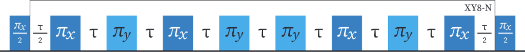
The XY8-N sequence is the most common DD sequences used for NV-based sensing and it consists of the following pulse sequence: \((\pi_x-\pi_y-\pi_x-\pi_y-\pi_y-\pi_x-\pi_y-\pi_x)^N\), where \(N\) is the so-called XY8 order and the indices \(x\) and \(y\) correspond to the rotation axis in the rotating frame. The pulses are spaced equidistantly with a spacing of \(\tau\), and applied after the spin is brought into a superposition state \(|-1> + |0>\). The entire sequence is shown in Figure 4a.

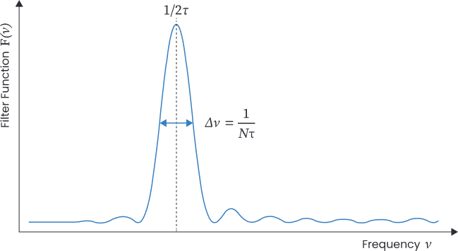
After the decoupling sequence, the spin state is mapped onto the spin population by a final \((\pi/2)_x\)-pulse. Finally, the NV center is read out optically by a laser pulse, which simultaneously repolarizes the electron spin state. Figure 4b shows the filter function of the sequence. The central frequency \(\nu=1/2\tau\) is defined by the periodicity of the pulses, while the width \(\Delta\nu=1/N\tau\) depends on the total acquisition time \(T=N\tau\).

---

Fig. 4a. XY8-N sequence with waiting time \(\tau.\)

---

Fig. 4b. Filter function of the XY8-N sequence. The central frequency is determined by the waiting time \(\tau,\) while the width is defined by the total acquisition time \(T=N\tau.\)

 

The example QUA program runs a for loop, which iterates through a given list of \(\tau\) values. Additionally, an outer for loop averages over many sweeps, as done in previous examples. We use the macro xy8_n(n) to create all the XY8 sequence pulses in a single line. The macro dynamically creates the XY8 sequence according to the order specified in parameter n, and it is written using a separate block macro xy8_block() for simplicity. The \(\pi_y\) pulses are generated by rotating the frame of the spin using the built-in frame_rotation() function. Then, the frame is reset back into its initial state by calling reset_frame().

# XY8-N Dynamical Decoupling sequence QUA code

with program() as xy8:
    avg_idx = declare(int) # averaging index
    i      = declare(int) # For XY8-N
    t      = declare(int) # For tau
    diff   = declare(int) # Diff in counts with reference
        play("laser_ON", "Laser")
    with for_(avg_idx, 0, avg_idx < N, avg_idx + 1):

        with for_(t, t_min, t <= t_max, t+dt): 
            play("pi_half", "Qubit") # XY8 sequence
            xy8_n(repsN)
            play("pi_half", "Qubit")
            times, counts = get_photons()

            play("pi_half", "Qubit") # XY8 reference
            xy8_n(repsN)
            frame_rotation(np.pi, "Qubit")
            play("pi_half", "Qubit")
            reset_frame('Qubit') 
            times_ref, counts_ref = get_photons()
        assign(diff, counts - counts_ref)


def xy8_n(n):
    wait(t, "Qubit")
    xy8_block()
    with for_(i, 0, i < n - 1, i + 1):
        wait(2 * t, "Qubit")
        xy8_block()
        wait(t, "Qubit")

def xy8_block():
    play("pi", "Qubit") # 1 X
    wait(2 * t, "Qubit")
    frame_rotation(np.pi / 2, "Qubit")
    play("pi", "Qubit") # 2 Y
    wait(2 * t, "Qubit")
    reset_frame("Qubit")
    play("pi", "Qubit") # 3 X
    wait(2 * t, "Qubit")
    frame_rotation(np.pi / 2, "Qubit")
    play("pi", "Qubit") # 4 Y
    wait(2 * t, "Qubit")
    play("pi", "Qubit") # 5 Y
    wait(2 * t, "Qubit")
    reset_frame("Qubit")
    play("pi", "Qubit") # 6 X
    wait(2 * t, "Qubit")
    frame_rotation(np.pi / 2, "Qubit")
    play("pi", "Qubit") # 7 Y
    wait(2 * t, "Qubit")
    reset_frame("Qubit")
    play("pi", "Qubit") # 8 X

For the NV centers optical readout, we utilize the macro we defined in a previous tab get_photons() which opens a time tagging window while triggering a measurement laser pulse. The same sequence is repeated a second time with a final \((\pi/2)_{-x}\). The photons detected during this are saved in the variable counts_ref and act as a reference signal.

At the end of each loop, we can save the photon counts and any other variable into a so-called stream (not shown here). These streams allow streaming data to the client PC while the program is still running. The stream processing feature also offers a rich library of data processing functions which can be applied to streams. The QOP server performs the processing before sending it to the client PC. It can significantly reduce the amount of transferred data by limiting it to the user’s preferred result.

Adding a Randomized Phase to the XY8 Sequence

A known issue with pulsed DD, is the emergence of spurious harmonics due to the pulses’ finite length. A theoretically “easy” solution is to introduce a random global phase to each iteration of the experiment [1]. This solution quickly becomes very taxing when trying to utilize it by a-priory waveform creation, because the number of repetitions we need to upload has to be very large (\(N\gg 100\)) for the phase to be considered random. As the OPX+ generates this sequence on the fly, we can utilize its internal random number generator to easily create this randomized XY8-N sequence by adding a couple lines of code to the one above. First, we will define an additional variable \(\phi\), then we add a line assigning a new random phase for each iteration using the command random().rand_fixed() which returns a random number between 0 and 1:

# Adding a randomized phase to the XY8 sequence
...  
phi = declare(fixed,value=0)
assign(phi,Random().rand_fixed()) 
play("pi_half", "Qubit") xy8_n(repsN, phi) 
...

The last step would be to add a frame_rotation() command before each \(\pi_x\) and reset_frame() at the end of the xy8_block() macro:

# Adding a phase commands to the XY8 sequence
...  
frame_rotation_2pi(phi, "Qubit")  
play("pi", "Qubit") # 8 X  
reset_frame("Qubit")  
...

frame_rotation() and reset_frame() are the tools that allow to have full and precise control of relative and absolute phase, comfortably and easily from QUA. By default, the OPX calculates the phase of each signal as if it started at \(t=0\), the beginning of the sequence. Thus, two outputs shooting sin waves at the same frequency will be phase-matching unless the user asks otherwise, by using these two frame control functions. Changing frequency back and forth will result in signals from different outputs still being phase-matched unless otherwise specified. Phase control has never been this easy.

Single-shot readout of a nuclear spin

One of the NV centers’ major strengths is its ability to utilize its nuclear spin environment as a quantum register for complex protocols that involve more than a single qubit (we again take NV as example, but it is the case for many defect centers and semiconducting or quantum photonics systems). This utility was already shown in many experiments, including quantum sensing [2,3], quantum computation [4], and quantum networks [5]. All these experiments share the need to initialize the nuclear spin to a known state, and efficiently readout that state via manipulation of the NV electron spin. We have shown a basic example of active reset in one of the previous tabs, but here we dive deeper on how codes look like in defect centers lab.

In order to actively initialize the nuclear spin, we first need to be able to determine its state, so we will first look at the single-shot readout (SSRO) [6]. As example we take an SSRO on the intrinsic \(^{14}N\) nuclear spin. The single-shot readout consists of a conditional rotation on the NV, a laser pulse to read its state, and then repeating these two steps \(N\) times to accumulate enough photons for state separation. As the \(^{14}N\) is a spin 1, two consecutive SSRO steps are necessary. In the first SSRO, the conditional \(\pi\) pulse will be performed if the nuclear spin is at the \(|0_N>\) sublevel. This will tell us whether the nuclear spin is at the \(|0_N>\) sublevel or at the \(|\pm1_N>\) sublevels. If we are at \(|0_N>\), the readout is done, if not, then a second SSRO needs to be initiated to determine whether the nuclear spin is at the \(|+1_N>\) or \(|-1_N>\) sublevel. The ability to skip the second SSRO step exemplifies the OPX+’s capabilities, as without real-time measurement-based decision making, one could waste precious nuclear spin coherence time on an unnecessary step. We write the SSRO protocol in a macro easy to reuse later. This macro sees conditional rotation, defined by the CnNOTe(), and then measurement.

We start with the C\(_n\)NOT\(_e\) gate on the electron spin. This gate inverts the electron spin only for a specific nuclear spin state. This is achieved by choosing the correct frequency in the hyperfine resolved ODMR spectra of the NV center (we have seen an ODMR code in a previous tab). In the QUA script below, the macro accepts the nuclear spin state for which the electron spin should be flipped as an integer (-1: \(|-1_n>\), +1:  \(|+1_n>\), 0:  \(|0_n>\)). It calculates the corresponding new intermediate frequency according to the given nuclear spin state by adding or subtracting the hyperfine splitting value (hf_splitting ≈ 2.16 MHz) from the central frequency \(f_0\) of the NV centers hyperfine spectra. We use the built-in QUA function update_frequency(), seen already before, to update the frequency applied to the element “Qubit”, which corresponds to the sensor spin. Finally, we play a \(\pi\)-pulse dynamically updating the pulse’s amplitude and duration and reducing the pulse’s frequency bandwidth.

# CNOT-gate macro for the electron spin - QUA code
def CnNOTe(condition_state):
    align() 
    update_frequency("Sensor", NV_IF + condition_state * hf_splitting) 
    play("pi_x"*amp(0.1), "Sensor", duration= (pi_length/4)*10) 
    update_frequency("Sensor", NV_IF) 
    align()

Once again, we re-use the get_photons() macro we have defined at the very beginning. It uses the command measure() with its time tagging capabilities to get the counts and timing of tags within a defined measurement window and save the information in real-time variables that the pulse processor can use right away, in the same sequence. Here, the macro runs in a for loop that runs for N times to accumulate enough photons for state differentiation. We compare total counts against a predefine SSRO_threshold. If lower, the nuclear spin is at the \(|0_N>\), and we can continue with the experiment. If higher, then we need to determine whether the nuclear spin is in the \(|+1_N>\) or \(|-1_N>\) states. This is done by repeating the SSRO, this time with the CnNOTe() receiving the integer 1. After the loop, we know the nuclear spin is at the \(|+1_N>\) if the photon count is lower than the threshold, and \(|-1_N>\) if it is higher.

def SSRO(N, result):
    i = declare(int) 
    ssro_count = declare(int,value=0) 
    with for_(i, 0, i < N, i + 1): 
         wait(100, "Sensor") 
         CnNOTe(0) 
         times, counts = get_photons() 
         assign(ssro_count, ssro_count + counts) 
         with if_(ssro_count < SSRO_threshold):
             assign(result, 0) 
         with else_():  
             assign(ssro_count, 0) 
             with for_(i, 0, i < N, i + 1):               
                 wait(100, "Sensor") 
                 CnNOTe(1) 
                 times, counts = get_photons()
                 assign(ssro_count, ssro_count + counts) 
                 with if_(ssro_count < SSRO_threshold):
                     assign(result, 1) 
                 with else_(): 
                     assign(result, -1)

Here we have used a hardcoded two-step process, but this process can also be written as a repeat-until-success protocol. We then would obtain a procedure of length not know a priori (not-deterministic), but can have it conditionally resetting until a certain arbitrary condition is met. For example, let’s assume we want to initialize the nuclear spin to a specific state (e.g. \(|0_N>\)). Instead of post-selection, which wastes time performing unwanted experiments or employing an elaborate SWAP gate (as it is a 3 level system), which takes a long time and usually has limited fidelity, the OPX+ enables the user to precisely perform the necessary operation based on the nuclear spin SSRO result.

In the case of nuclear spin initialization, we would start, like above, with a SSRO on the \(|0_N>\) sublevel. If the nuclear spin is at that level, we are done. If not, a second SSRO is performed to determine whether the nuclear spin is at the \(|+1_N>\) or \(|-1_N>\). Based on the result of the second SSRO, an RF \(\pi\)pulse on resonance with the desired transition can then be applied on the nuclear spin to bring it back to the \(|0_N>\). If a \(\pi\) pulse was performed, we can repeat the process to make sure the nuclear spin is in the desired state. The code example is written in the init_nuclear_spin(), which starts with the SSRO() macro to initially determine the nuclear spin state. Then, if it is not in the \(|0_N>\), the code enters an indeterministic while loop, until the SSRO() determines the nuclear spin is in the \(|0_N>\) state. After each SSRO, a selective \(\pi\) pulse will be applied to the nuclear spin with a frequency determined by the result of the SSRO.

# Nuclear spin initialization using repeat-until-success QUA code 
def init_nuclear_spin():       
    state = declare(int)       
    SSRO(N_SSRO, state)       
    with while_(state == ~0):            
        with if_(state == -1):                 
            update_frequency("Memory", memory_IF_m1)                 
            play("pi_x", "Memory")                 
            update_frequency("Memory", memory_IF_p1)            
        with else_():                 
            play("pi_x", "Memory")                 
            SSRO(N_SSRO, state)

Nanoscale NMR with a nuclear spin memory

With the OPX and QUA, we can write even the most complex experiments as short and clear single programs. To demonstrate this, let’s look at an NV center-based NMR experiment that utilizes a nuclear spin as an additional memory [2,3]. It is possible to drastically enhance the spectral resolution by using the long lifetime of the nuclear spin as a resource. This technique allows nanoscale NMR with chemical contrast, e.g. [7]. We use, a setup similar to Figure 1, seen a few tabs back, where an OPX orchestrates Laser pulses, MW and RF signals, but also readout from the NV center in diamond.

NMR using NV center qubits is typically based on imprinting the Larmor precession of sample spins into the phase of a superposition state of the NV electron spin state [8]. We can achieve this, for example, by using Ramsey spectroscopy, Hahn echo sequences or dynamical decoupling (some of which we have seen before). The spectral resolution of these methods is limited by the duration of the phase accumulation period, and consequently, is limited by the coherence time \(T_2^{sens}\) of the sensor spin. It’s possible to overcome this limitation by performing correlation spectroscopy [9] . Here, the signal is generated by correlating the results of two subsequent phase accumulation sequences separated by the correlation time \(T_C\). During the correlation time, the phase information is stored (partially) in the polarization of the sensor spin. Hence, the possible correlation time, and therefore the spectral resolution, is limited by the spin-relaxation time \(T_1^{sens}\) (\(>T_2^{sens}\)) of the sensor.

Fig. 5. A sequence of NMR with memory spin. It consists of active initialization of the memory spin, encoding, sample manipulation, decoding, and a final readout of the memory spin via single-shot readout.

It’s possible to improve this even further by utilizing a memory spin, which has a much longer longitudinal lifetime (see sequence in Figure 5). In the correlation spectroscopy experiment we discuss here, the information is stored on the nuclear spin (memory) instead of on the NV spin (sensor). As a result, the achievable correlation time is significantly increased. The intrinsic nitrogen nuclear spin of the NV center is a perfect candidate to act as this memory spin. It is strongly coupled to the NV center electron spin, which acts as the sensor, while its coupling to other electron or nuclear spin is negligible. When applying a strong bias magnetic field (3T) aligned along the NV-axis, we can achieve memory lifetimes \(T_1^{mem}\) on the order of several seconds. In this example, we assume that the used NV center incorporates a 14N nuclei with a 1-spin and the eigenstates \(|+1_n>\), \(|-1_n>\) and \(|0_n>\).

Figure 5 shows the complete sequence. It consists of five steps: initialization, encoding, sample manipulation, decoding, and readout. For initialization and readout, we use the macros SSRO() (which includes CnNOTe() ) and init_nuclear_spin(), that are described above, so we won’t repeat them here. Here, we build a macro for each of the other steps, which act on three elements (connected each to an output channel): “Memory”, “Sensor” and “Sample”:

# QUA code for encoding step of NMR sequence in Fig 5
def encode(t):
     align()
     reset_frame("Memory")
     play("pi_2_x", "Memory")
     CnNOTe(0)
     wait(t // 4, "Sensor")
     CnNOTe(0)
     play("pi", "Sample")
     CnNOTe(1)
     wait(t // 4, "Sensor")
     CnNOTe(0)
     play("pi_2_y", "Memory")
     align()

The encoding aims to encode the sample sensor interaction into the spin population of the memory spin. First, the memory spin is brought from its initial state \(|0_n>\) into a superposition state by a \(\pi/2\)-pulse. Next, entanglement between sensor and memory is established for two phase-accumulation windows. The entanglement is created and destroyed by nuclear spin state selective \(\pi\)-pulses performed on the sensor spin. While the sensor and memory spins are entangled, the interaction with the sample spins leads to a phase accumulation on the memory spin superposition state. In between the two phase-accumulation periods, the sample is actively flipped by a resonant \(\pi\)-pulse. The final phase \(\Delta\phi=\phi_2 – \phi_1\), where \(\phi_1\) and \(\phi_2\) are the accumulated phases during the first and second accumulation window respectively, is then mapped into the memory spin population by a final \(\pi/2\)-pulse on the memory spin. The decoding sequence is identical, except for the conditions of the C\(_n\)NOT\(_e\) gates on the sensor spin.

# QUA code for decoding step of NMR sequence in Fig 5
def decode(t):
     align(*all_elements)
     play("pi_2_x", "Memory")
     CnNOTe(1)
     wait(t // 4, "Sensor")
     CnNOTe(0)
     play("pi", "Sample")
     CnNOTe(1)
     wait(t // 4, "Sensor")
     CnNOTe(1)
     play("pi_2_y", "Memory")
     align()

Now that we have all of the building blocks we can write a QUA program to perform the entire sequence in Figure 5:

# QUA code for decoding step of NMR sequence in Fig 5
N_avg = 1e6           # Number of averages
N_SSRO = 5000         # Number of readouts
hf_splitting = 2.16e6 # N14 hyperfine splitting 
t_e = 2000            # Time of encoding/decoding
SSRO_threshold = 200  # Readout threshold
all_elements = ["Sensor", "Sample", "Memory"]
tau_vec = [int(i) for i in np.arange(1e3, 5e4, 5e3)]
with program() as prog:
    avg_idx    = declare(int)  # average index
    tau        = declare(int)  # time to vary
    result_vec = declare(int, size=len(tau_vec)) 
    c = declare(int)

    with for_(avg_idx, 0, avg_idx < N_avg, avg_idx + 1):
        assign(c, 0)
        with for_each_(tau, tau_vec):
            init_nuclear_spin()
            encode(t_e)
            align(*all_elements)
            play("pi_2", "Sample")
            wait(tau, "Sample")
            play("pi_2", "Sample")
            align(*all_elements)
            play("laser", "Sensor")
            decode(t_e)
            SSRO(N_SSRO, result_vec[c])
            assign(c, c + 1)
            with for_(n, 0, n < result_vec.length(), n + 1): 
                save(result_vec[n], "result")

The QUA-function align(), already discussed in previous examples, is used to define the timing of the individual pulses. One of the basic principles of QUA is that every command is executed as early as possible. Hence, when not specified otherwise, pulses played on different quantum elements are played in parallel. To ensure that pulses play in a specific order, we use this built-in function for temporal alignment. This function causes all specified quantum elements to wait until all previous commands are complete, and so it aligns them in time.

The main script runs the whole sequence for different values of the waiting time of the Ramsey sequence played on the sample spin in a for loop. Additionally, the experiment is averaged over N_avg repetitions by an outer loop. The result for each value of is saved into the corresponding item of the result vector result_vec.

The ease of use of QUA and the capabilities of the OPX and its PPU allow to write advanced sequences such as this in a matter of minutes. It is very common to see quantum photonics labs performing all calibrations, characterization and all advanced quantum circuits in mind, in just the first few days of operation. Have a look at this blog post to see what a typical 48 hours installation looks like.

I hope this dive into examples for optically addressable qubits (with NV center qubits as spotlight example) was interesting. I am sure now you have more questions than before starting to read. So it is a good time to contact us for a virtual demo, where you can ask us live questions on how to perform the most advanced sequences you have in mind. You will find the challenge button here or below, so what are you waiting for? Request a Demo.