
QM’s Orchestration Platform for
Quantum Sensing
Run advanced quantum-sensing protocols with synchronized optical, microwave, RF, and photon-detection control. QM’s Orchestration Platform enables programmable dynamical decoupling, nanoscale NMR, adaptive readout, and real-time feedback for sensors that respond to the world while the measurement is running.


QUANTUM SENSING
Research
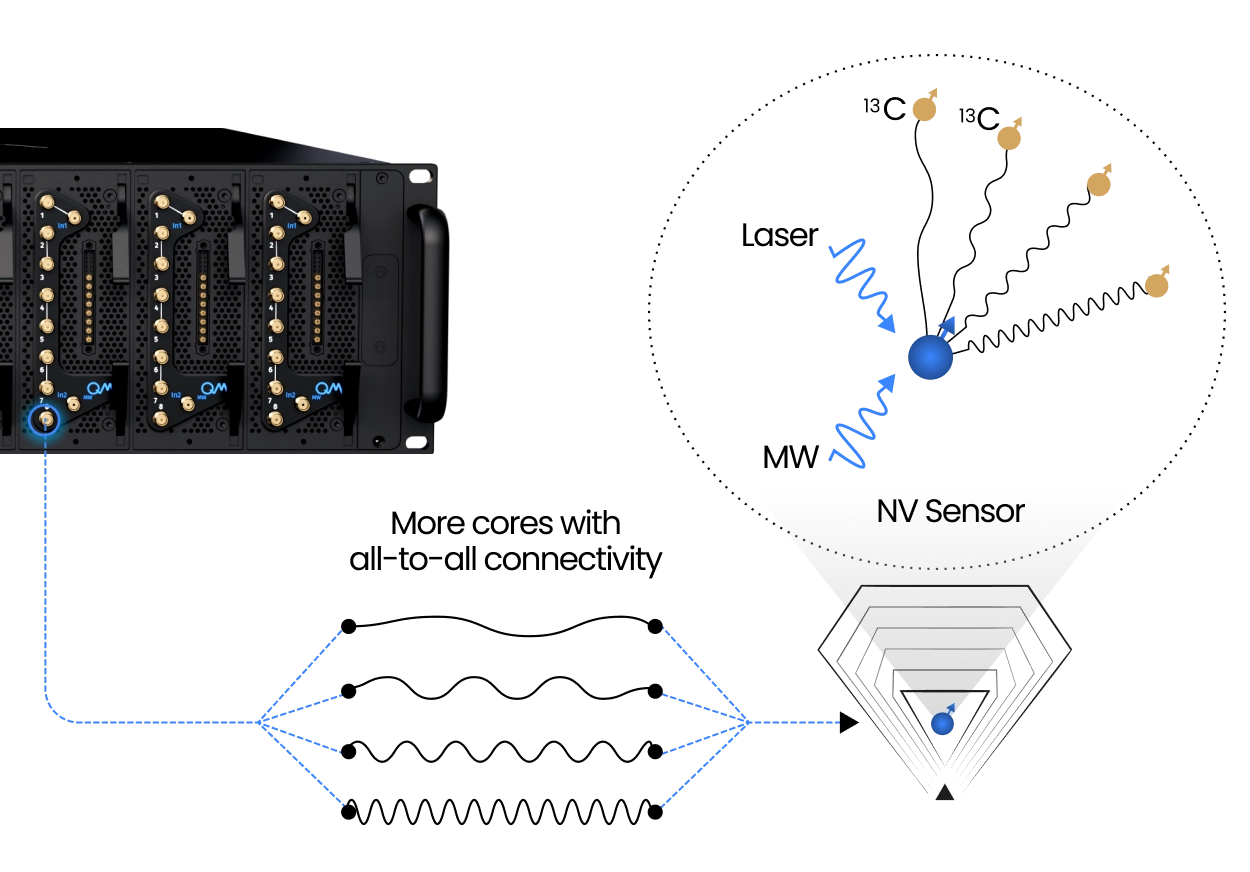
Quantum sensors use the sensitivity of quantum systems to measure magnetic fields, temperature, strain, electric fields, and nearby nuclear or electronic spins with exceptional precision. Platforms such as NV centers and other Defect Centers are especially powerful for nanoscale sensing and imaging because they combine optical addressability, long coherence, and operation across practical experimental conditions. As sensing protocols become more advanced, they require precise optical, microwave, RF, and photon-detection control, often across long and highly structured pulse sequences.
Quantum Machines’ Orchestration Platform supports advanced quantum-sensing experiments by synchronizing laser excitation, spin control, photon time tagging, and real-time feedback from one platform. With OPX hybrid controllers and QUA, researchers can program dynamical decoupling, nanoscale NMR, multi-frequency spin addressing, QND readout, and adaptive sensing workflows that update parameters while the measurement is running. This helps teams move from fixed pulse execution to responsive experiments that extract more information from every shot.
Programmable Dynamical Decoupling for Quantum Sensors
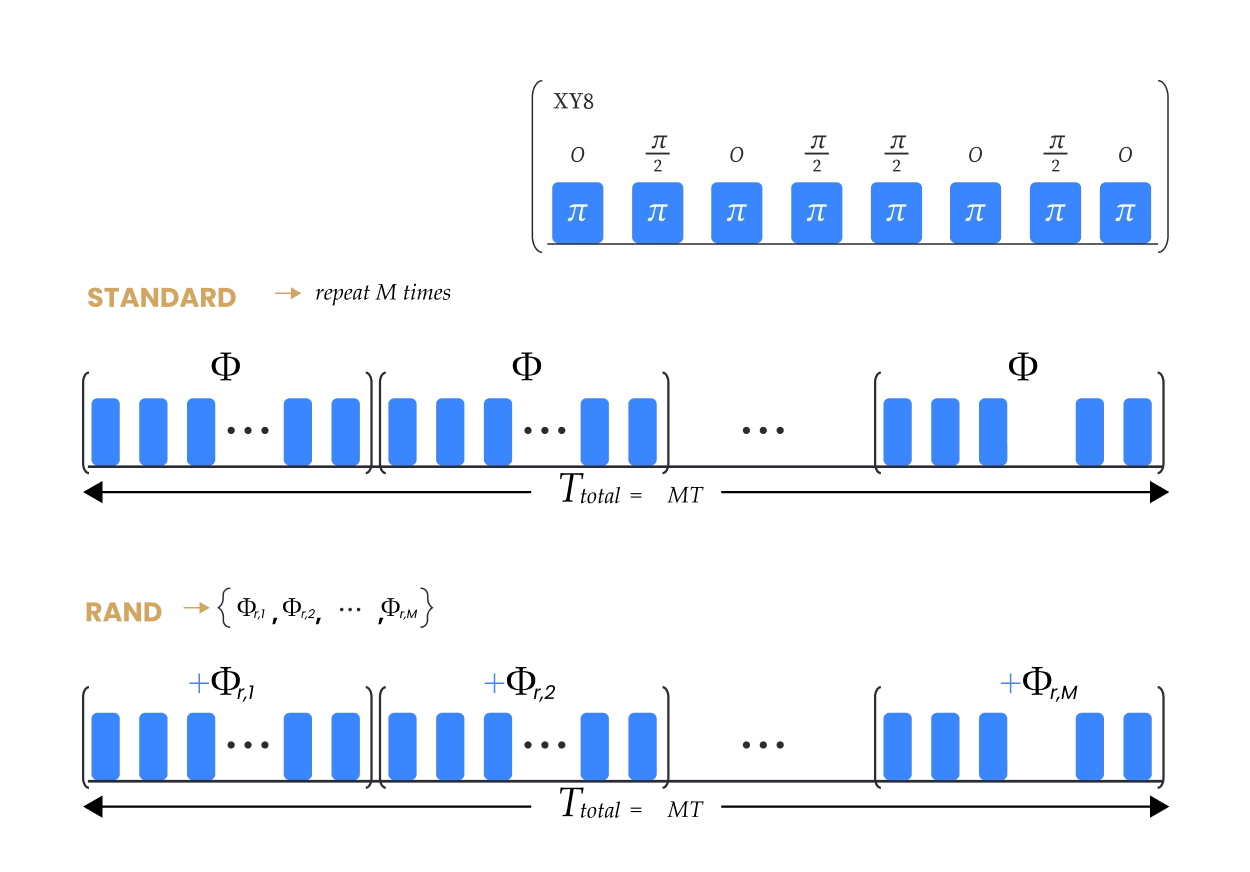
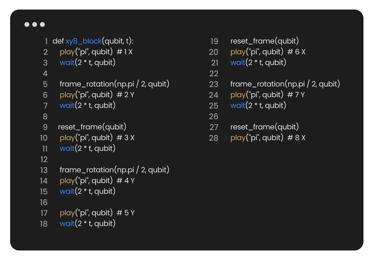
Advanced quantum sensing often relies on long, structured pulse sequences that protect coherence while making the sensor selectively sensitive to signals of interest. Dynamical decoupling protocols such as XY8 act as programmable frequency filters, enabling measurements of weak magnetic fields, nanoscale NMR signals, and environmental noise spectra. QM’s Orchestration Platform lets researchers build these sequences directly in QUA, using reusable macros, real-time loops, phase control, and synchronized optical readout. Instead of uploading long static waveforms, OPX executes pulse instructions on the controller, making extended sensing protocols easier to modify, repeat, and scale while preserving precise timing across microwave, RF, laser, and photon-detection channels.
Nanoscale NMR and Multi-Frequency Spin Addressing
Quantum sensors can probe nearby nuclear spins with nanoscale resolution, but doing so requires precise control of both the sensor spin and the target spins. Protocols such as DDRF interleave RF pulses with electron-spin dynamical decoupling, enabling individual nuclear-spin addressing while preserving coherence. QM’s Orchestration Platform synchronizes microwave, RF, optical, and photon-detection channels within a single pulse-level workflow. With OPX and QUA, researchers can update RF frequencies, preserve phase across pulse blocks, multiplex multiple tones, and run parallel spin-control macros directly on the controller. This makes complex nanoscale NMR and multi-spin spectroscopy experiments easier to program, stabilize, and extend.
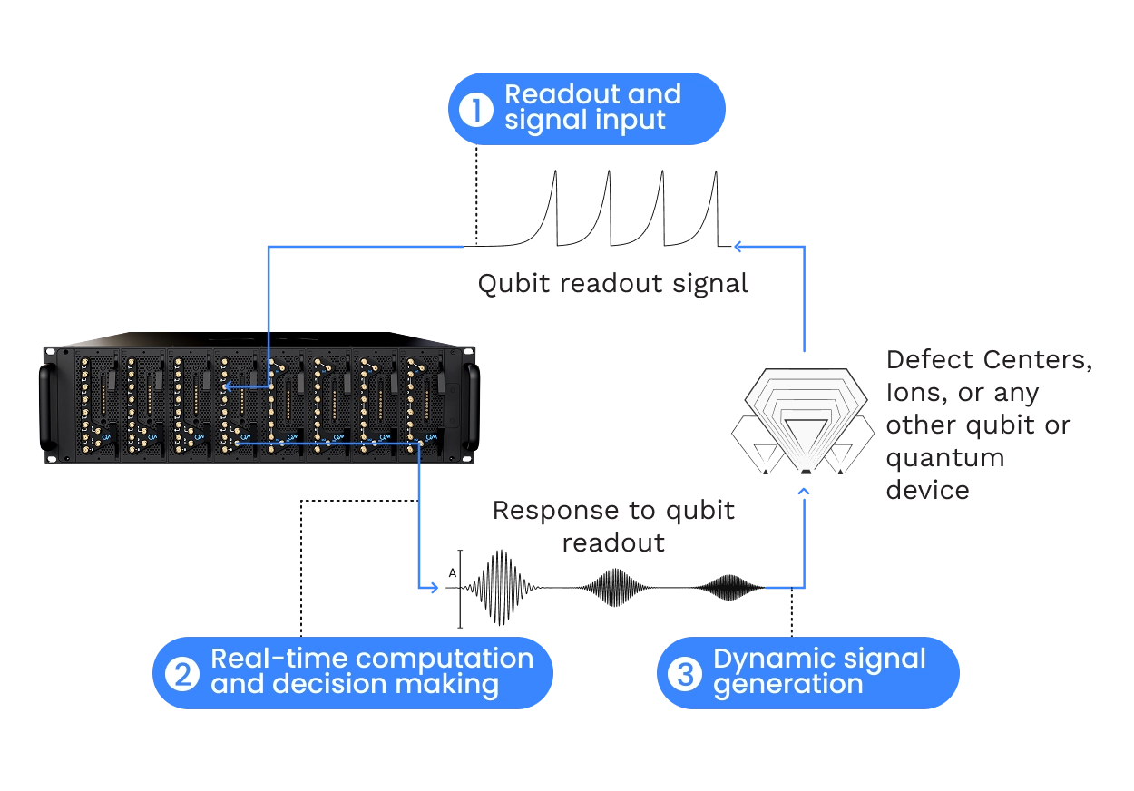
Adaptive Sensing with Real-Time Photon Processing
The most sensitive quantum-sensing protocols are rarely static. Measurements may need to extend until enough photons are collected, update thresholds, narrow a frequency range, track drift, or change the next pulse based on the signal already observed. QM’s Orchestration Platform enables these adaptive workflows by processing photon counts, time tags, and measurement outcomes in real time. With OPX and QUA, sensing sequences can branch conditionally, update pulse parameters, decide whether to repeat or continue, and apply feedback without waiting for offline post-processing. This supports QND readout, correlation spectroscopy, long-coherence measurements, and experiments where every shot and every photon can improve sensitivity. Such capabilities are key value for Quantum Sensing, but also Quantum Networks applications. Read an example of time-tagging-based feedforward in Ruskuc, A., Nature 639, 54–59 (2025).
Replacing 3 devices with one synchronized, orchestrated machine tremendously simplified lab workflow. Now our pulse sequences run in a fraction of the time of any other device combo. Plus, we can “talk” to the FPGA in human-speak, to run real-time calculations that were too complicated before! Along with the yoga-level


FAQs
How does the platform run dynamical-decoupling sequences like XY8?
Dynamical-decoupling protocols act as programmable frequency filters, making a sensor selectively sensitive to weak magnetic fields, nanoscale NMR signals, or noise spectra while protecting coherence. QM lets researchers build these in QUA using reusable macros, real-time loops, phase control, and synchronized optical readout. Rather than uploading long static waveforms, the OPX executes pulse instructions on the controller, so extended sequences are easy to modify, repeat, and scale with precise timing across all channels.
How does QM enable nanoscale NMR and multi-frequency spin addressing?
Probing nearby nuclear spins requires controlling both the sensor spin and the target spins, which protocols like DDRF achieve by interleaving RF pulses with electron-spin dynamical decoupling to address individual nuclei while preserving coherence. The platform synchronizes microwave, RF, optical, and photon-detection channels in one pulse-level workflow. With OPX and QUA, researchers can update RF frequencies, preserve phase across pulse blocks, multiplex multiple tones, and run parallel spin-control macros directly on the controller.
What makes adaptive sensing possible on the platform?
The most sensitive protocols may extend until enough photons are collected, narrow a frequency range, track drift, or change the next pulse based on the signal already seen. The OPX enables this by processing photon counts, time tags, and measurement outcomes in real time, so sequences can branch conditionally, update parameters, and decide whether to repeat or continue without offline post-processing. This supports QND readout, correlation spectroscopy, and long-coherence measurements where every shot and photon improves sensitivity.
Do I need separate time taggers or correlators for quantum-sensing experiments?
No.Photon counting and time tagging are native to the controller, so external instruments aren’t required. These capabilities can be implemented in a few lines of code without external switch trees or stand-alone electronics such as time taggers, drivers, or correlators, and any measurement result can be used immediately to change outputs within hundreds of nanoseconds. That keeps the full sensing loop from excitation, to detection, to decision and feedback, all on one platform.