Active Reset for Qubits: Building Qubits You Can Count On
Quantum computing with superconducting qubits promises speed, scale, and new physics. But none of these promises hold if qubits start out in the wrong state.
That’s why active reset qubits are essential for reliable and scalable quantum computing.
Typically, we aim for the qubits to start in the ground state, with as low as possible residual excitations in thermally excited states. Without this clean starting point, every computation carries hidden errors before the first gate is even applied. This becomes even more essential as systems scale – when ancilla qubits must be reset every cycle, often thousands of times per second. If that reset isn’t fast and reliable, reset errors can affect the logical error rates. This is where qubit reset protocols come in, tackling this challenge by ensuring precise qubit initialization in every cycle.
Qubit reset protocols: many paths to initialization
One of the simplest ways to reset qubits, perhaps, is the thermal one. However, simple does not mean efficient nor effective. Thermal reset relies on the following principle: if you let systems be, they will eventually thermalize, leading to ground states with higher probability, compared to active reset approaches. For superconducting qubits, the time for this to happen is 5 to 10 times the qubits’ energy relaxation time (T₁).
This is a problem. As we scale towards fault tolerant quantum computing (FTQC), we strive to make qubits with longer T₁ times and faster error correction and mid-circuit protocols. Thermal reset loses on both fronts.
Thermal reset for superconducting qubits requires waiting for 5-10 times the T₁ time for the qubit and is a stochastic process. Even though the relaxation rate is the same, each qubit undergoes decay at a random time. For large-scale QPUs this is not a suitable option as it makes mid-circuit measurements impossible to achieve.
With state‑of‑the‑art QEC cycles at 1.1 µs and qubits with 70µs T₁ times, thermal reset becomes the main bottleneck and would end up consuming more than 99% of the cycle time. Besides being slow, thermal reset is a stochastic process. Even if the qubit has a well defined relaxation rate, individual qubits do not relax to the ground state at the same time. The fidelity of the process is ultimately limited by the thermal population distribution. That means that passively waiting for thermal reset is not an option.
The solution is a smarter reset.
Measurement-based active reset for qubits
Dispersive measurements map qubit states onto distinct state-dependent phase shifts in the resonator readout tone, producing separate clusters in the phase plane. This measurement-based active reset protocol enables fast and reliable qubit initialization. Tighter integration between quantum and classical resources, including real-time classical computation and control flow, reframes the problem of resetting qubits as a measurement, feedback and action task on the data in the phase plane.
We measure the state of the system and play pulses that set the qubit state conditioned on the measurement result above or below a predetermined threshold. If the value is above the threshold, indicating greater likelihood of being in the excited state, we play a π pulse to bring it to the ground state. If it is below, we do nothing. However, doing this at nanoseconds latency, as is needed for QEC cycles, is not trivial. First, measuring the state of a superconducting qubit comes with its own uncertainty. The state of a qubit is measured by the phase of the signal from the readout resonator. Depending on the state of the qubit, we get two different values of the phase.
Since the measurements are noisy, each qubit state produces a Gaussian distribution of possible measured phases. A single measurement is just one noisy sample from that distribution, so repeated shots land in the same Gaussian but at different points. The Gaussians, as shown below, overlap in a region making state discrimination uncertain. From the control perspective, a feedback-based protocol for reset must be capable of discriminating the measurements based on a threshold and then apply a control logic flow in real-time. This is what OPX1000 is built for, bringing reset times down to 200 ns – best in the industry by far.
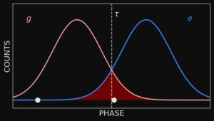
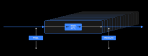
Top: the image shows the control flow for the active reset process. Bottom: The image shows two Gaussians representing the likelihood of the qubit in states |g⟩ and |e⟩ based on the phase value. The single threshold allows for deciding when to apply the conditional π pulse. The shaded area under the Gaussian represents the misclassified states and ultimately limits the fidelity.
In the simplest type of measurement-based active reset, the threshold is set at the intersection of the two Gaussian distributions. If the phase is smaller than the threshold value, then stay put. If the phase is greater than the threshold, apply a π pulse to bring it to the ground state. However, in the region of overlap, this protocol can lead to false positives or false negatives. Beyond the tail ends, we can be fairly confident of the state of the qubit from the measured value. But in the overlap region, a measurement lying above the threshold when the qubit is in the ground state would falsely trigger a π-pulse creating an excited state error. Conversely, a measurement falling below the threshold when the qubit is in the excited state is falsely classified as being in the ground state and is left uncorrected.
Repeat until success (RUS) qubit reset protocol
One way to tackle this is another reset protocol called repeat until success (RUS) reset. In RUS, instead of one threshold, we use two, as well as repeated active reset sequences to improve fidelity of initialization. The first threshold (𝜏₁) is set at the tail end of the blue Gaussian and the peak of the red Gaussian. The other threshold (𝜏₂) is set at the point of intersection of the two curves. The presence of the two thresholds can now address the false results.
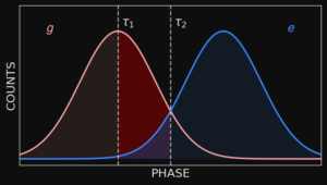
Top: The image shows the control flow for the RUS process. The image shows repeat until success protocol with two thresholds. The first threshold decides when to exit the reset protocol while the second threshold decides when to apply the conditional pi pulse. When the value is between the thresholds, the measurement process is repeated until the value falls under the first threshold. Bottom: The two thresholds on the Gaussians are shown. Depending on where the two thresholds are placed, more of the misclassified states can be correctly characterized.
If the measurement is below 𝜏₁, we know that the qubit is in the ground state (and 𝜏₁ can be moved arbitrarily to the left, trading time for higher fidelity). We can then call the qubit initialized and proceed with our experiments. If the measurement is above 𝜏₂, the probability of being in the excited state is higher and we apply a π pulse to reset the qubit and measure again.
However, if the measurement falls between 𝜏₁ and 𝜏₂, there is high uncertainty about the state of the qubit and we repeat the measurement. Repeated measurements can have instances of measured phase that fall below 𝜏₁ or above 𝜏₂, resolving the uncertainty issue. This cycle repeats itself until the measurement is below 𝜏₁, in the ground state up to readout fidelity. If we choose 𝜏₂ to be at the tail end of the red Gaussian and the peak of the blue Gaussian, the fidelity can be further improved, but it comes at a cost of time. In this way, successive measurements reduce uncertainty and improve fidelity compared to a basic active reset protocol. Still, RUS is inherently non-deterministic – it relies on repeating until the measured phase is below the thresholds.
For a system with many qubits, it means that the time to reset qubits can vary. While some qubits are getting reset, there may be others that are already reset but remain idle and prone to reheating. The above-mentioned protocols use static thresholds to perform conditional operations. For scaling, both protocols have limitations. Active reset has poor state discrimination, and RUS is time non-deterministic. Adaptive reset protocols can address both of these challenges. Adaptive reset protocols rely on the fact that every measurement has information content that can be used to redefine what we know and don’t know about the system, even if the system is uncertain.
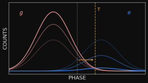
Top: the image shows the control flow for the adaptive reset process. The image shows the reset process with a threshold that is updated per iteration. The adaptive threshold, computed from all the priors from the measurements, allows for deciding when to apply the conditional π pulse. By setting the number of times we perform this iteration, this process can be adapted for scalable QPUs. Bottom: The Gaussians indicating the probability of the system being in the ground or excited state are updated at each round. This in turn evolves the threshold as shown.

