Introduction to Digital Filters 02: Correcting IIRregularities

Written in collaboration with Gal Winer and Uri Abend

The business of manipulating signals is right at the core of qubit handling, and it is not trivial. Nature has decided that all those little imperfections that make life interesting also corrupt our perfect electrical signals. Fortunately, since the Quantum Orchestration Platform (QOP) relies on a digital processor inside the OPX to generate pulses, we have access to the power of digital filters to help correct some of our misfortunes. If you’re a theoretician, you can forget about this and move on with your carefree life.  But if you’re an experimentalist like me, I am afraid you’ll have to tag along.

In general, the path our signals go through to reach our qubits will introduce delays and dispersion, distorting the shapes we send. It does not matter how well you simulate the perfect pulses if you don’t account for setup frequency-dependent response. This realization marks the moment we ask ourselves if doing theory wasn’t the better option. In this blog post, we will strive to avoid this question, and instead, we will discuss how we deal with discrepancies and instrument responses in correcting our qubit-control signals.

We use two main types of digital filters to this end, both supported by the QOP. The first is Finite Impulse Response (FIR) filters which are used to correct signals with only knowledge of the input, so a feed-forward operation. We discussed these in this FIR filters blog post, so check it out. The other type is the Infinite Impulse Response (IIR) filters, which modify signals depending on both input and output, thus also performing feedback. Those are what we focus on today.

WHO BROKE MY SQUARE PULSE?

The main idea is to measure the effect of our path towards the qubit, including all components, and then pre-distort our perfect pulses to compensate for this measured response. The major distortion component often comes from one or two elements, like bias-T, that we can disconnect and measure separately. In this simple case, we shoot a square pulse, read what comes out, and then distort the input pulse until we get a square pulse out. This is a simplification, but you get the idea. In other cases, the components are many or cannot be easily disconnected (e.g., inside the fridge), so people use the cryoscopy technique to monitor discrepancies in signals going through the experimental setup.

Once calibration is done, you know that every time you want to shoot a pulse, you have to distort it in some calibrated way to compensate for that component’s response. In the old days, like five years ago (remember, time in physics research moves ~25 times faster than regular time), people used to load each and every corrected pulse and sequence, point by point, into a wave generator memory to perform experiments. 

Today, we can leverage the real-time computation of the QOP architecture to separate our sequence design and the correction. Once the filters are calibrated, you can forget about system response, trusting that all signals will be corrected on the fly just before leaving the OPX output. No hassle and no memory issues. If we want to send a square pulse to our qubit, the processor only needs two numbers, amplitude and duration. Correction is automatic. This freedom is as close as we will ever get to doing theory.

IIR BASICS FOR COOKS

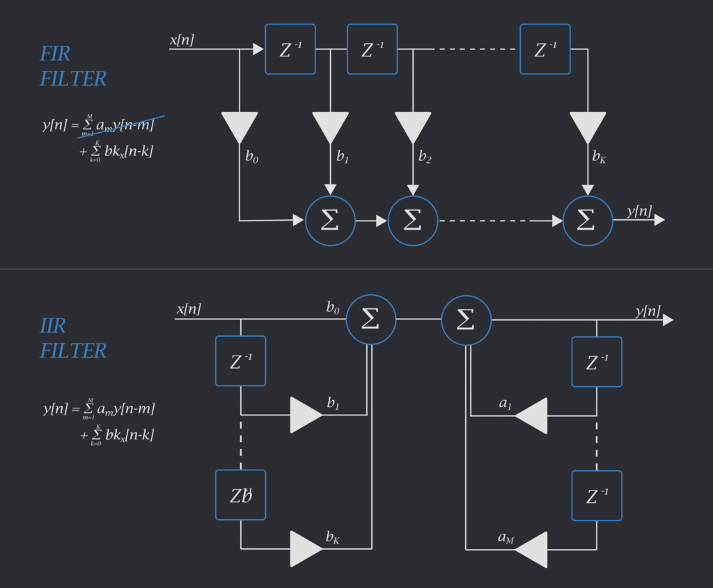
IIR are the cool kids of the filters’ neighborhood. In contrast with FIR, IIR filters also imply a sort of memory effect for outputs instead of just inputs, so the output depends on the previous output. In general, a filter can be written as:

Where \(y[n]\) is the output in time and \(x[n]\) is the input. k going from 0 to K refers to the indexes of past and present inputs, while m going from 1 to M refers to indexes of past outputs. In our previous FIR post, we introduced the term tap, which is just a coefficient in Digital Signal Processing (DSP) terms. So \(a_m\) and \(b_k\) are the feedback and feedforward taps, respectively. If the first term of the equation, which depends on the past outputs, is not zero, then we are talking about IIR filters. Hopefully, Figure 1 will clarify this a little.

Let’s try to go out of the math realm to understand the difference between FIR and IIR. Let’s say we are cooking dinner—one dinner per day, seven days a week. Every day we choose the meal to prepare based on what’s in our fridge. Until we go to the store to buy more food, each meal decision will depend on what we have used as inputs in the previous meals (do we still have carrots?). So we need a memory of past ingredient usage. This analogy explains the FIR filter setting when the filter’s output is an arbitrary combination of past inputs.

Continuing our analogy, there’s a giant broccoli field just next to our garden. So while it’s hard to keep track of broccoli usage, we have plenty. With our previous method, we might end up making broccoli salad for weeks! Instead, we remember what we have eaten previously, and add that information to our considerations. So if over the past few days we decided to have a broccoli salad, we’ll factor in this output for our next decision, and we might decide to avoid broccoli. For this, we also need a memory of past outputs. And this is the setting of an IIR filter.

Now, I will probably end up in the lowest circle of the DSP Hell for the inaccuracies of wild cooking metaphors. Nonetheless, I think stirring things up could help us swallow the concept.
See what I did there?

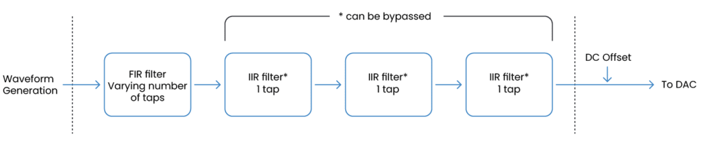
For those more interested in technical stuff, IIR filters allow us to model both zeros and poles in the transfer function of our filter. The OPX+ has 3 IIR filters in sequence before each DAC, each of which has one tap and can be individually bypassed, so from zero to three poles. If used, they add from \(48\,ns\) to \(72\,ns\) in delay to all outputs, while allowing you to correct even very long setup imperfect responses. IIR filters are particularly well-suited for correcting exponential decays, such as bias-T.

FLUX LINES: CORRECTING OUR BIASES(-T)

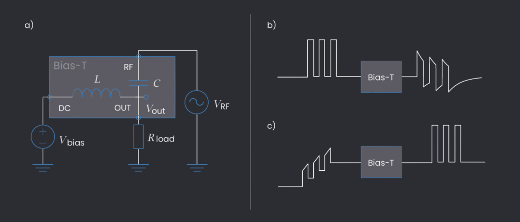
In many quantum labs where qubits reside, we use bias-T setups to combine DC and RF signals in one line. This is often done for transmon qubits, quantum dots, and others. In a bias-T (see Fig. 2a), even if we assume infinite internal impedance of the DC source (simplified version, but most often reasonable), the load and the capacitance act as an analog RC first-order high-pass filter on the RF input. So if we send a train of square pulses, this gets distorted by passing through the bias-T (see Fig. 2b).

The correction can be done with an FIR filter, but in case of a very long response to correct, we would need to handle way too many taps (e.g., microsecond response times lead to thousands of taps necessary for FIR). IIR filters in cascade offer an efficient alternative. This is slightly different from having one IIR with many taps (as shown for the general case in Fig. 1) but allows efficient cumulative taps and reduces computation overhead when dealing with multiple components. Each IIR feedback tap allows correcting for one pole, hence one resistor-capacitor pair, one bias-T.

The case we have seen here is the so-called DC-block. Just to give you an idea of how the math looks like, its response function is provided by:

Which we can correct with its inverse Laplace transform (we use it to convert from analog to digital):

So yay! We can calculate what correction our square pulse train needs in order to actually be a square pulse train after the bias-T. As we can see, all that matters is the time constant of the resistor-capacitor pair, and this can be measured or often found in spec sheets. We show an example of how this would look in Fig. 2c.

IIR FILTERS WITH OPX & QUA

Implementing IIR (and FIR) filters in QUA is straightforward and done in the configuration file for analog outputs. The filter is applied individually for each output and can be bypassed if not necessary. The OPX+ has three IIR filters in cascade, with one tap each.

By setting the taps, the filter is automatically configured to one of the following modes:

• Bypass mode — disables the filter and sets its output to be its input.
• FIR mode — supports M=0 and K=43.
• IIR mode — supports M=1, K=36 OR M=1 2-times, K=29 OR M=1 3-times, K=22.

While the configuration is straightforward (in this case with feedback taps only):

"analog_outputs": {
        1: {
            "offset": 0, 
            "filter": {"feedforward": [], 
            "feedback":[0.5, -0.3, 0.1]}},
            },

Adding a filter to any port will delay all analog pulses coming out from all ports and delay feedback operations. The OPX synchronizes all outputs, so you don’t have to think about the relative time between outputs. This default synchronization can be turned off for more advanced applications.

SUMMING UP

With its 44 FIR taps and the 3 IIR taps, reconfigurable and bypassable, the OPX+ covers virtually all filtering needs of a qubit lab. It offers correction for zeros and poles of imperfect setup response functions with the minimal latency between \(44\,ns\) and \(73\,ns\), depending on the number of taps used. You can set the OPX to bypass unused filters to completely remove latencies and keep the highest performance. Once you finish with the filter settings, you can altogether forget about corrections. Each output will be modified according to your configuration, and programs will remain filter-agnostic and straightforward.

With this, we conclude our introductory series on digital filters. But stay tuned, as we will soon show some great customer results demonstrating how people are using these DSP capabilities on their setups. If you’re interested in reading more or even finding some useful QUA code snippets, please visit our GitHub repository for some interesting examples!