How is The OPX Different to General Purpose Equiptment?

Are the Fischer lines twisted in QSwitch?

Yes, they are twisted all the way through the PCB in the configurations 1-2, 3-4, …, 23-24, identical to the twisted pair wiring in our Fischer cables.

What is the bandwidth of QSwitch?

The bandwidth is significantly larger than the QDAC-II bandwidth. Measured from a BNC input through a 3m Fischer output cable, the bandwidth is larger 5 MHz. Please note that the overall bandwidth in an experimental setup will most likely be limited by the impedance match of the in-series connected devices.

Is QSwitch an all-to-all switch matrix?

No, it cannot be used to change the configuration of the Fischer lines from input to output (e.g. input line 23 to become output line 21). But one can say: QSwitch’s 240 software-controlled relays offer maximum flexibility to connect any Fischer line to a Fischer input or any of 8 BNCs for monitoring and control. 

Can QSwitch be used without the Fischer input?

Absolutely, yes.

What is QSwitch and what does it do?

QSwitch is an easy-to-use, software-controllable breakout box for quantum labs that saves valuable research time. By remote controlling experiments and removing the need for cable adjustments, QSwitch makes the last manual lab operations obsolete. QSwitch’s 240 software-controlled relays offer maximum flexibility. You can connect any Fischer line to a Fischer input – or to any of 8 BNCs for monitoring and control. 

Pre-program experiments and quickly switch between setups and instruments – without touching anything. Work remotely with full visibility of routing. Control, log, and oversee all signal paths using Python scripts – with only minutes of set-up time. 

QSwitch has ultra-low noise, with minimal crosstalk – and minimal switching transients for reliable qubit operation. It’s also easy to integrate with other instruments – and to set up in the rack. Automatic soft grounding keeps valuable equipment safe during power outages. 

What is the isolation to ground of QBox signal lines?

Every QBox is tested at 100V to have a minimum isolation of 17 GOhm between signal lines and ground.

Are there filters inside QBox and can they be configured?

QBox does not have any built-in filters. We have kept it simple to reduce complexity, especially when debugging the measurement setup. At the same time, we have left plenty of space between the BNC connectors so that in-line filters can be placed there. 

How does QBox work?

In the breakout box each signal line is routed from the 24-pin Fischer connector to a BNC connector. This is done in shielded twisted pairs. Small switches enable grounding signal lines individually or connecting them to a common BNC, allowing for the same voltage to be set on multiple lines. The spacing between the BNC connectors on the front panel is large enough for in-line filters or BNC-T pieces.

I have a system with more than 24 lines. How can I scale QFilters?

For systems requiring more than 24 lines, QFilters can be efficiently stacked, saving space on the mixing chamber plate, or connected in series, removing the need for jumper cables. This flexibility allows for configurations like dual RC or dual RF filters, catering to diverse setup requirements.

What is the standard configuration for QFilter?

Our standard configuration offers two filtering banks (low-frequency and radio frequency) with 25-pin micro-D connectors. These banks are connected in series using a shielded jumper cable. The compact, non-magnetic design allows for direct mounting on the mixing chamber plate and is compatible with most fridge manufacturers, such as Bluefors fridges and the Oxford Instrument Proteox. 

What is the QFilter and what does it do?

QFilter-II is a compact solution for advanced multi-stage low-pass filtering. It’s specifically designed to reject noise and maintain millikelvin electron temperatures across 24 signal lines. It reduces electron temperature through filtering to typically 5-15 mK above the mixing chamber. This makes it an ideal fit for quantum electronics devices and other sensitive cryogenic circuits. Originating from extensive research at Harvard University and the University of Copenhagen, QFilter is now a trusted tool in over 100 research groups worldwide. 

Is QCage.24 light-tight?

QCage is enclosed in a light-tight superconducting EMC shielding enclosure.

Does QCage.24 fit in a standard BlueFors sample loader?

QCage.24 is supplied with brackets to replace the mounting rods, making it fit in the 80mm BlueFors sample loader. It bolts onto the mounting rail, and the QCage.24 should be configured with cables going to SMP connectors.

Does QCage.24 fit in a standard Oxford puck? 

QCage.24 is designed to fit in the newer Oxford 72/73 mm pucks, specifically the 144 mm long variant with mounting rods spaced by 56.2 mm. It can be mounted either centrally or in top or bottom positions by positioning the supplied 25 mm extension rods. For puck mounting, QCage.24 should be configured with cables going to SMP connectors.

What are the relevant microwave losses in the QCage?

The overall loss has been verified from open-ended reflection measurements to be less than 3 dB to 20 GHz. We have made the following budget to account for the different sources of loss: 

• Cable loss ≈ 1.4 dB (product data) 
• Connector loss ≈ 0.2 dB (product data) 
• Sample board loss, less than 1 dB (combined connector-to-line matching and bulk dielectric losses) 

Note that additional losses will be introduced from wire bonding and matching to the on-chip transmission line circuit. 

Is the QCage.24 sample board made of a superconducting PCB?

No, the sample board is made as a copper stack, four layers with low-loss dielectric between. The signal-carrying paths are configured as 50 ohm coplanar transmission lines in one of the buried layers. To ensure common microwave grounding, vias are placed in a dense pattern along the lines, which also helps to thermalize the four layers. Finally, the copper is plated by a non-magnetic nickel-free gold plating to prevent oxidation, provide better thermalization, and assist with easier wire bonding.

What sample thickness fits in QCage.24? 

The intended thickness is 525 µm (standard for 4-inch wafers). The suspended pedestal height will work for sample thickness ranging from 475 um to 575 µm. For thinner sample thickness, we provide a metal spacer to place under the chip with an 8 x 8 mm clearance area. For thicker sample thickness, we provide a metal spacer to place under the PCB. Both are 125 µm thick and can be stacked to support any sample thickness ranging 225 µm to 950 µm. 

What sample size fits in QCage.24? 

The cavity of the QCage.24 sample holder is 10.5 x 10.5 mm, designed to support chip sizes ranging 10 x 10 mm +/- 0.5 mm. Chip sizes smaller than 9.5 x 9.5 risk falling through the corner pedestals. For smaller chip sizes, we can provide adaptor plates for 5 x 5, 6 x 6, and 7 x 7 mm. These will fit chip sizes ranging + 0.2 mm / – 0.4 mm.

What is QCage.24?

QCage.24 is a microwave cavity-based sample holder system for transmission line measurements with a 24-way interface optimized up to 18 GHz. It relies on having the sample chip suspended in the cavity, separated from the boundaries to minimize losses and decoherence. Further, it has an EMC tight superconducting shielding and an optional flux biasing magnet inside the shielding. As such, the QCage presents a versatile and high-performance sample holder system, particularly for superconducting qubit experiments with 10 or more qubits.

What fridges are compatible with QBoard-II?

A versatile set of mounting brackets ensures full compatibility with Oxford (Proteox and Triton), as well as Blufors (60×300, 80×300) fridges. A universal mounting bracket is also available for custom integration.

How does QBoard-II ensure optimal signal quality?

QBoard-II minimizes RF losses and reduces crosstalk, ensuring the quality of your measurements and experiments. Offering radiation protection for both the quantum chip and electrical components, QBoard-II comes with a new shielding lid. The lid fully encloses the sample for proper radiation protection and shields the RC filter components for the lowest noise environment.

What new features does QBoard-II have, compared to the original QBoard?

QBoard-II features more compact dimensions; new PCB, interposer, and daughterboard designs; and the addition of a shielding lid. The upgraded design with 16 high-density RF and 48 low-frequency RC lines enables transmission from DC to 8 GHz. The new PCB design minimizes losses and crosstalk. This is useful for applications such as readout of superconducting resonators, sub-nanosecond gate-voltage pulses, and high-bandwidth frequency sweeps. It enables an easy upgrade with unchanged connector configurations.  

What is QBoard-II and what does it do?

QBoard-II is a modular, PCB-based sample holder system that supports low-temperature experiments with spin-qubits, superconducting circuits, and general transport measurements. QBoard-II supports any experiment from simple fast turnaround sample characterization to complex microwave-powered experiments. It is an ideal interface to operate qubit quantum processors with up to eight spin qubits. 

What are phase coherence and noise in quantum sequences, and how do they impact qubit fidelity?

Phase coherence refers to the stability of the phase relationship between signals over time, which is crucial for accurate qubit manipulation and information transfer. Phase noise, on the other hand, is a random, unpredictable, and irregular fluctuation seen on any given signal individually. This noise can disrupt not only the coherence between channels but also the operation each pulse is supposed to implement on the qubits. Digital Direct Synthesis (DDS) plays a vital role in minimizing noise and maintaining phase coherence, thereby enhancing qubit fidelity and the reliability of quantum computing systems.

How does DDS impact the speed and efficiency of quantum algorithms?

Digital Direct Synthesis (DDS) can significantly impact the speed and efficiency of quantum algorithms by providing precise, fast, and flexible control over qubits. This precise control allows for quicker execution of quantum operations and algorithms, improving overall system performance. Additionally, the high coherence of DDS-generated signals helps obtain high qubit fidelities, directly influencing the efficiency of quantum computing operations.

How does Digital Direct Synthesis (DDS) contribute to the scalability of quantum computing systems?

Digital Direct Synthesis (DDS) contributes to the scalability of quantum computing systems by offering a flexible and programmable method for generating control signals. Its digital nature allows for easier integration with other digital components and systems, facilitating the development of larger, more complex quantum computing architectures without compromising on performance or increasing the system’s footprint significantly.

What is the spurious-free dynamic range (SFDR), and how does it relate to Digital Direct Synthesis (DDS) and mixer calibration?

The spurious-free dynamic range (SFDR) is a measure of a system’s ability to generate a waveform without unwanted signals or harmonics that could interfere with the signal. In Digital Direct Synthesis (DDS) systems, a high SFDR is crucial for ensuring that the generated waveforms are clean and free from unwanted noise. This is particularly important in quantum computing, where signal purity directly impacts qubit fidelity.

What are the main performance metrics for microwave waveform generation?

The main performance metrics for microwave waveform generation include frequency bandwidth, phase noise, spurious-free dynamic range (SFDR), and spectral purity. These metrics determine the ability of a system to generate precise and clean waveforms, which are essential for accurate qubit manipulation.

How does Digital Direct Synthesis (DDS) compare to mixer-based solutions like IQ mixers, sideband mixers, or double super-heterodyne (DSH) conversion?

Digital Direct Synthesis (DDS) provides a more straightforward and precise approach to generating and controlling waveforms than mixer-based solutions. While IQ mixers, sideband mixers, and DSH conversion methods can offer flexibility in frequency generation, they often require complex calibration and can introduce additional noise and distortion. DDS, on the other hand, directly generates clean, low-noise signals, simplifying the setup and enhancing performance in a scalable manner.

What are the advantages of using Digital Direct Synthesis (DDS) over traditional analog signal generation methods?

Digital Direct Synthesis (DDS) offers several advantages over traditional analog signal generation, including:

1. Higher resolution and real-time programmability of frequency, phase, and amplitude.
2. Lower phase noise and better signal stability.
3. Greater flexibility in waveform generation without the need for complex hardware changes.
4. Improved scalability and integration capabilities with digital systems, crucial for complex quantum computing setups.

Can Digital Direct Synthesis (DDS) be used to control multiple qubit types, and if so, how?

Yes, thanks to Digital Direct Synthesis (DDS), the MW-FEM offers a wide frequency range and can accomodate operations on many qubit modalities. It enables multi-tone drive and full real-time control of any pulse parameter, including phase. These capabilities allow for the precise manipulation of different types of qubits, such as superconducting qubits or trapped ions, within the same quantum system. This versatility is achieved through the programmability of DDS, which can tailor signals to the specific resonance frequencies and control requirements of each qubit type.

What are the key components of a Digital Direct Synthesis (DDS) system in quantum research?

A typical Digital Direct Synthesis (DDS) system in quantum research comprises a high-resolution frequency synthesizer, a digital-to-analog converter (DAC), a phase accumulator, a digital waveform generator, and a low-pass filter. These components work together to generate accurate and stable waveforms that can manipulate qubits with high precision, and they are all seamlessly integrated in the MW-FEM module of the OPX1000.

What is Digital Direct Synthesis (DDS), and how does it apply to quantum computing?

Digital Direct Synthesis (DDS) is a method for generating precise and stable microwave waveforms digitally. In quantum computing, DDS is utilized to produce the microwave pulses needed to manipulate or readout qubits. It offers a programmable, high-resolution method to control the quantum states with minimal noise, which is crucial for maintaining the coherence of qubits over time.

What are the challenges in implementing quantum communication?

Key challenges include maintaining quantum state integrity over long distances, scaling the technology for widespread use, and developing interoperable standards between quantum and classical communication systems.

What are the primary differences between quantum communication and classical communication?

Quantum communication utilizes quantum states for transmitting information, enabling inherently secure communication through quantum encryption, unlike classical communication which relies on classical physical signals.

What are the major challenges in quantum networking and how are they addressed?

Challenges include maintaining quantum coherence over long distances, efficient error correction, and integrating quantum and classical networks. Solutions involve advanced quantum repeater technology and robust quantum control protocols, that leaves the heavy lifting on the control electronics orchestrating the sequence.

How does entanglement distribution work within a quantum network?

Entanglement distribution involves creating entangled qubit pairs and transmitting them to different quantum network nodes, enabling quantum communication and computation over long distances.

What are the fundamental components required to build a scalable quantum network?

Key components in building a scalable quantum network include quantum repeaters for extending range, entanglement sources, quantum routers for directing information, and quantum memories for storing quantum states. Such diverse components must be orchestrated from a single unified controller able to perform real-time calculations and decision making.

What are the advantages of optically addressable qubits over electrically addressable ones in quantum computation?

Optically addressable qubits offer advantages like lower interference and crosstalk, higher precision in control, and potentially faster operation speeds, crucial for efficient quantum computation.

How does optical addressing of qubits affect the overall performance of a quantum computer?

Optical addressing allows for precise control of qubits with minimal crosstalk, leading to higher fidelity in quantum operations and potentially increased quantum computing performance.

What techniques are used to achieve optical addressing of individual qubits in a quantum system?

Optical addressing techniques include using laser beams focused on individual qubits, exploiting differences in qubit resonance frequencies, and employing optical cavities to enhance interaction with qubits. For high speed and scalable operation the challenge falls on the control system that orchestrates the sequence.

How can we generate and manipulate single photons for quantum photonic applications?

Efficient generation and manipulation of single photons can be achieved through advanced techniques like spontaneous parametric down-conversion, quantum dot emitters, and integrated photonic circuits, ensuring precise control and minimal loss. These techniques, combined with a control system able to orchestrate sequences in real-time, allow to code and compute quantum operations.

What are the main challenges in integrating quantum photonic devices into existing optical networks?

Integration challenges of quantum photonics include ensuring compatibility with classical network infrastructure, maintaining quantum coherence over long distances, and developing interfaces for efficient quantum-classical information conversion.

How do quantum photonic systems differ from classical photonic systems?

Quantum photonic systems utilize the principles of quantum mechanics, like superposition and entanglement, allowing them to perform tasks that are impossible in classical systems, such as secure quantum communication and enhanced sensing. They also have different requirements from the perspective of the control electronics, to allow for integrated quantum and classical operations.

How do photonic quantum processors compare to other types of quantum processors in terms of speed, accuracy, and scalability?

Photonic quantum processors offer faster operation speeds and are less sensitive to environmental disturbances, enhancing accuracy. However, scalability remains a challenge due to complexities in controlling large numbers of photons. Thus, the scalability issue becomes a requirement for the control electronics, which must be reliable and performing, even when controlling large scale quantum systems.

What are the main applications for photonic quantum processors?

Photonic quantum processors are ideal for applications in quantum communication, quantum cryptography, and quantum simulation, especially in scenarios requiring high-speed operations and stability against environmental disturbances. Given the high-speed logic required, it is recommended to have access to a smart real-time controller to orchestrate the sequences.

What are the key challenges in building scalable and error-resistant photonic quantum processors?

Major challenges include minimizing photon loss, ensuring high-fidelity quantum gate operations, scaling the system while maintaining coherence, and developing quantum error-correction methods specific to photonic systems. Quantum-classical processing and a smart controller that orchestrates the entire experiment in real-time can greatly mitigate the challenge.

How does a photonic quantum processor encode and process information using photons?

Photonic quantum processors use photons as qubits to encode information. These photons are manipulated using optical elements like mirrors, beam splitters, and phase shifters to perform quantum computations through processes like interference and entanglement. To control the photon generation and manipulation process, it is recommended to use an orchestration system with real-time processing, baseband and/or microwave drive, depending on experimental needs.

Can I do time tagging with the OPX platform?

Yes, and much more! Time tagging and TTL counting are key elements of many quantum computing platforms (e.g., NV centers, optically addressable and quantum photonic systems, and AMO) and can be performed with OPX – QM’s advanced quantum control platform . Signals coming out of single-photon counting modules (SPCMs, or similar) can be directly connected to the OPX+/OPX1000 inputs, and tagging/counting is then performed natively within the Pulse Processing Unit. OPX+/OPX1000 users employ this technique for a great deal of different applications, such as optical quantum sensing, communication, and quantum information processing. As such, counting & tagging are key components of our solution.

The OPX standard operational mode time-tags events with 1 ns timing resolution with 1 ns dead time, for each of the analog input channels. Additionally, a high-resolution time tagging mode is available, pushing the resolution down to a few tens of picoseconds (~50ps) with increased (<100ns) deadtime. Check out the newest features of the OPX!

A time-tag is generated when a voltage trigger edge is detected at one of the analog inputs. The trigger edge can be defined in configuration and can be a simple threshold or an arbitrarily complicated dynamic multi-threshold, polarity, and derivative check. This allows you to easily implement complicated sequences spending virtually no time in setting up your time tagging configuration. Then, the time tagging is done easily within a measure command in a single line:

times = declare(int, size=10)
counts = declare(int)
measure([pulse],[element],[stream], time_tagging.analog([times],[duration],[counts])

This approach is universal and is fully embedded in the real-time logic of the PPU. Therefore, a time tagging command will allow for results to be used in real-time during an experiment, e.g. setting dynamic thresholds, performing estimations on the fly, or for conditional triggers. This could mean sending out a trigger pulse to a laser only if and when a signal is time-tagged and recognized as satisfying a certain threshold. It could also mean performing Bayesian estimation on a vector of tags, updating it while new tags come in. This is done with the smallest latency possible (on the order of ~100 ns for the simplest case), as all computation, tagging, and decision making is done in real-time on the FPGA-based pulse processor. 

The ability to write complex sequences with only a few lines of code while retaining the full performance of the FPGA ensures ease of use and the fastest time to result. Coding a dynamic Bayesian estimation protocol on a real experimental setup just became a first-year programming exercise. This makes life in the quantum photonic computing (NV center qubits and more) much simpler.

In the QOP framework, time tagging is one of many tools that can be used for real-time branching, computation, and control. All of the analog inputs of the OPX+ allow for flexible and independent time tagging capabilities, while our next-generation product high-density quantum control platform, the OPX1000, will offer many more inexpensive digital input channels, to be used for the experiments with many digital signals involved.

How can I program multi-channel sequences with the OPX+?

The OPX+’s Pulse Processor is a multi-core processor. Each pulser core executes its own sequence independently of the others, unless a protocol calls for inter-core dependencies. Synchronizing and coordinating different threads is handled by the compiler behind the scenes, making it easy to set up complex experiments with simple instructions.

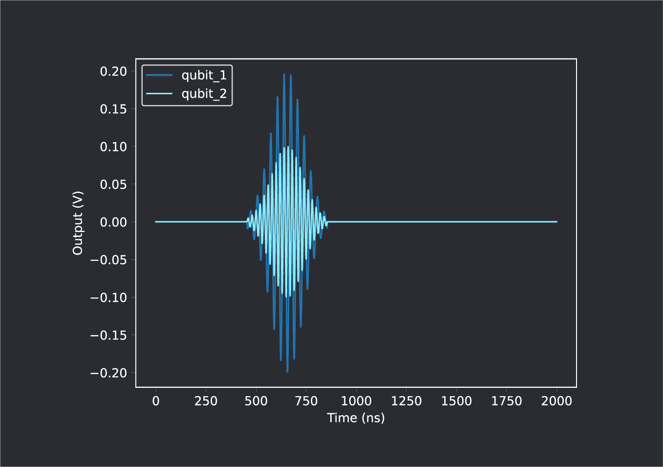
Suppose we want to play a Gaussian pulse with amplitude A1 to qubit_1, simultaneously with another Gaussian with amplitude A2 to qubit_2. This would be done with the following QUA program:

play(‘gaussian’*amp(A1), ‘qubit_1’)
play(‘gaussian’*amp(A2), ‘qubit_2’)

The two play() commands address different threads, and therefore play simultaneously. This results in an output as shown below:

We can delay one of the pulses by using the wait() command. In the following code, the qubit_1 thread alone is delayed by 20 clock cycles, while the qubit_2 thread is unaffected:

wait(20,’qubit_1’)
play(‘gaussian’*amp(A1), ‘qubit_1’)
play(‘gaussian’*amp(A2), ‘qubit_2’)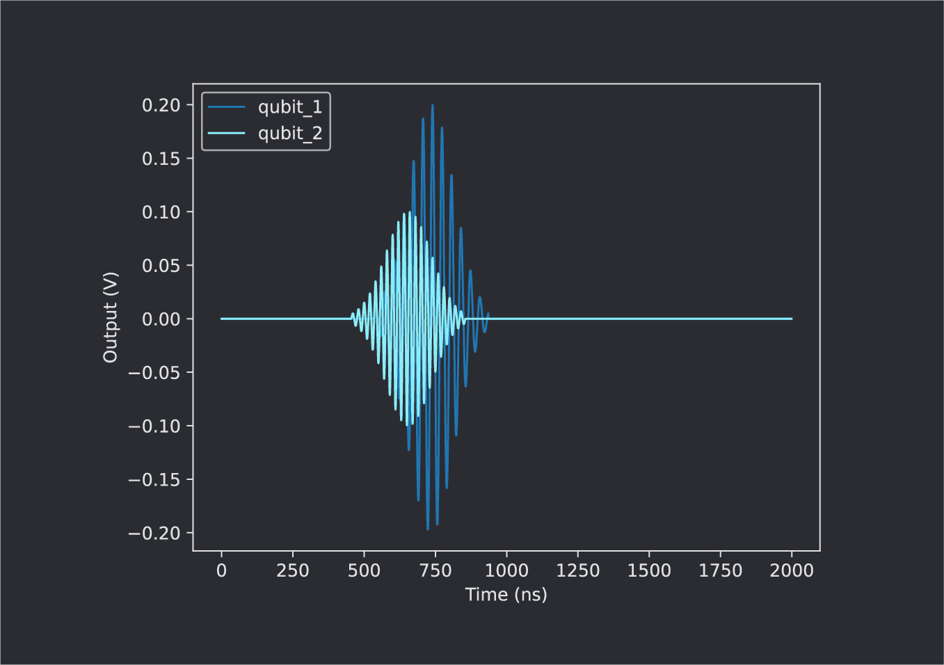

Many experiment protocols call for one sequence to begin only after another sequence is finished. Rather than manually calculate the duration of the first sequence, this can be implemented in QUA with the align() command:

play(‘gaussian’*amp(A1), ‘qubit_1’)
wait(20,’qubit_1’)
play(‘gaussian’*amp(A1), ‘qubit_1’)
align(‘qubit_1’, ‘qubit_2’)
play(‘gaussian’*amp(A2), ‘qubit_2’)

This results in the following output:

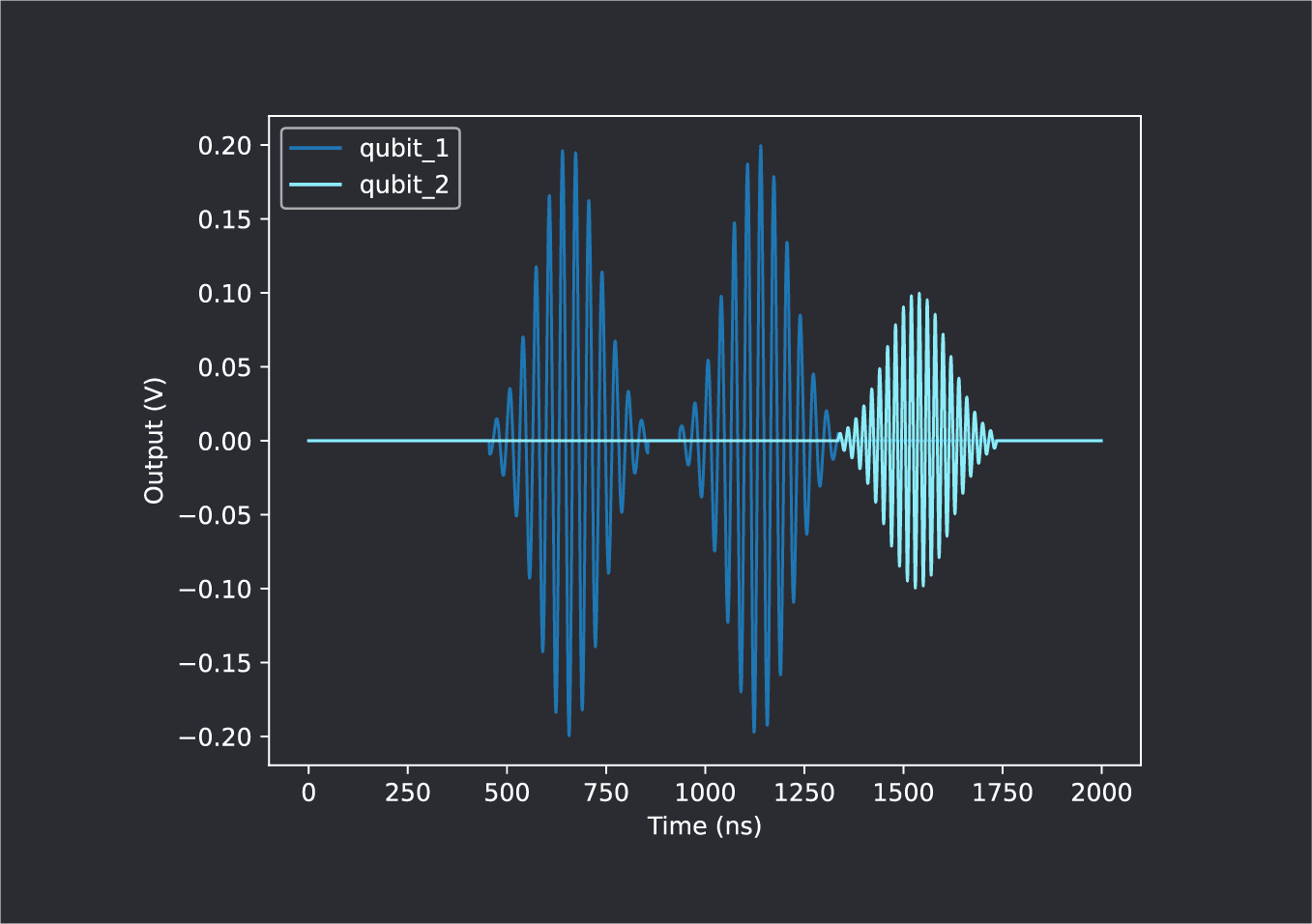
The align(‘qubit_1’, ‘qubit_2’) command causes the two threads to wait for each other. Any command appearing below this line that addresses either of the two threads will only be implemented after both have completed all commands appearing above this line. This dependency is evaluated in real time, and synchronizes the threads even if the duration of the first sequence is not known at compile time!

This last point is vital for many sequences, such as repeat-until-success protocols. Consider the following code:

with while_(result>0.2 && N < 1000):
          ### Subroutine involving ‘qubit_1’ ###
          align(‘qubit_1’, ’qubit_2’)
          play(‘gaussian’*amp(A2), ‘qubit_2’)

This will run a nondeterministic while() loop, within which the OPX+ might play pulses to qubit_1, measure it, update the result variable based on the measurement, and increment the counter variable N. It might run a single iteration before exiting the loop, and it might run 1,000. This is not known at compile time. But the simple align() still synchronizes the pulses, with all of the real-time control complexity handled by the compiler.

Why use a new quantum programming language, QUA, and how do I use it?

Well, there’s the long and the short of it. So let’s start with the short:

Why: Because we’ve built it to operate as quickly, efficiently, and easily with the Pulse Processor, giving you an adaptive, intuitive, and fully controllable way to probe your qubits. 

How: Surprisingly easily!

Now, let’s get into the heart of the matter:

As physicists, we understand the pain of having to learn yet another programming language, but writing FPGA and low-level code every time you want to run a Ramsey measurement? That’s a worse kind of pain. How many lines of code do you need to painstakingly write in order to run the experiments of your dreams? Probably more than you care to admit. This is where QUA comes in. QUA is a pulse-level quantum coding language that allows quantum researchers to run any experiment, on any type of qubits, quickly and easily. That Ramsey pulse, for instance, can be written, sent, and measured in just 10 lines of QUA code. But more on that in a minute.

When designing QUA, we set out to find the easiest way to program our pulses and send them to the qubit. We wanted to create a direct line of communication with our FPGA-based Pulse Processor in the OPX+, allowing us to have complete control of everything we might want. This quantum language was built by quantum physicists for quantum physicists, all with the purpose of making your quantum experiments as seamless as can be.

You write QUA the way you would explain it to other physicists in your group. You play this pulse to that element, listen on this measurement channel, demodulate that result. 

As for how the language actually works, there are three main steps: define a pulse sequence, play that pulse sequence, and measure the readout of that pulse sequence.  

The piece-de-resistance is that the compiler does all of the hard work: translating the pulses to FPGA commands. In other words, you need to program only on the high-level pulse programming language QUA, which is translated into the low-level FPGA. Programming in such a way is very useful; imagine you want to generate parametric Gaussian wavefunctions. With an AWG, you would need to upload a bunch of Gaussian profiles and figure out the timing in between. With QUA, you can set a for loop, which loops over various Gaussian amplitudes, sequentially. Turning your experiment into instructions that the FPGA can understand and run is already taken care of.

Feel free to check out this blog post with more info on QUA and the OPX+. And here is a quick guide covering the essentials of QUA.
Do feel free to reach out to us if you would like any more insight or information on how we can help you perform your experiments.

Can I implement real-time analog feedback with the OPX+?

Well, there’s the long and the short of it. So let’s start with the short:

Why: Because we’ve built it to operate as quickly, efficiently, and easily with the Pulse Processor, giving you an adaptive, intuitive, and fully controllable way to probe your qubits. 

How: Surprisingly easily!

Now, let’s get into the heart of the matter:

As physicists, we understand the pain of having to learn yet another programming language, but writing FPGA and low-level code every time you want to run a Ramsey measurement? That’s a worse kind of pain. How many lines of code do you need to painstakingly write in order to run the experiments of your dreams? Probably more than you care to admit. This is where QUA comes in. QUA is a pulse-level quantum coding language that allows quantum researchers to run any experiment, on any type of qubits, quickly and easily. That Ramsey pulse, for instance, can be written, sent, and measured in just 10 lines of QUA code. But more on that in a minute.

When designing QUA, we set out to find the easiest way to program our pulses and send them to the qubit. We wanted to create a direct line of communication with our FPGA-based Pulse Processor in the OPX+, allowing us to have complete control of everything we might want. This quantum language was built by quantum physicists for quantum physicists, all with the purpose of making your quantum experiments as seamless as can be.

You write QUA the way you would explain it to other physicists in your group. You play this pulse to that element, listen on this measurement channel, demodulate that result. 

As for how the language actually works, there are three main steps: define a pulse sequence, play that pulse sequence, and measure the readout of that pulse sequence.  

The piece-de-resistance is that the compiler does all of the hard work: translating the pulses to FPGA commands. In other words, you need to program only on the high-level pulse programming language QUA, which is translated into the low-level FPGA. Programming in such a way is very useful; imagine you want to generate parametric Gaussian wavefunctions. With an AWG, you would need to upload a bunch of Gaussian profiles and figure out the timing in between. With QUA, you can set a for loop, which loops over various Gaussian amplitudes, sequentially. Turning your experiment into instructions that the FPGA can understand and run is already taken care of.

Feel free to check out this blog post with more info on QUA and the OPX+. And here is a quick guide covering the essentials of QUA.

Do feel free to reach out to us if you would like any more insight or information on how we can help you perform your experiments.

How much pulse memory is available to store waveforms?

The OPX+ uses memory in a completely different way from your garden-variety AWG, and we should first understand how so as not to compare apples to oranges.

Consider how you would play a Ramsey sequence from an AWG with a 1 GSPS sampling rate. This involves uploading a waveform long enough to contain the two excitation pulses as well as the delay in between. If each pulse is 20 ns long, and the delay between them is 1000 ns, then at a sampling rate of 1 GSPS this waveform would consist of 1040 samples.

The OPX+ pulse processor operates in a completely different manner. Firstly, only the pulse amplitude is stored in the memory; upconversion to the intermediate frequency happens in real time. A pulse of constant amplitude and arbitrary length is thus generated from a single sample!

For the Ramsey sequence we might want the 20 ns pulse to have a Gaussian envelope, and accordingly use 20 samples of waveform memory. The QUA program to run a Ramsey sequence would look like this:

play(“Gaussian”,”Qubit”)
wait(t_delay)
play(“Gaussian”,”Qubit”)

The OPX+ uses the same waveform memory to play the Gaussian twice, and can just as easily play it a thousand times — with the same 20 samples! In fact, it can dynamically change the Gaussian amplitude, or stretch the Gaussian for a pulse duration longer than 20 ns — whether pre-programmed or in a real-time response to measurement — without using additional memory.

What about the wait(t_delay) command? An AWG requires a long sequence of zeros to space the pulses, and since characterization of high-coherence devices require long delay times, memory limitations can be prohibitive. But in the OPX+ the wait() command does not use any waveform memory!

A full Ramsey experiment, including a measurement operation followed by a wait() command to allow the qubit to return to the ground state, would look like this:

with for_each_(t_delay, t_values):
        play(“Gaussian”,”Qubit”)
        wait(t_delay)
        play(“Gaussian”,”Qubit”)
        measure(“Readout”,”Qubit”,...)
        wait(reset)

The array t_values over which we are looping for t_delay can contain a million values, and the variables t_delay and reset can have values of seconds — and the entire experiment will still exploit the same 20 samples of waveform memory.

Now that we understand how powerfully and intelligently the OPX+ utilizes its memory, we can give a short answer: Each OPX+ channel has a waveform memory of 2^16 = 65,536 samples. This sounds small for an AWG, but is huge for a pulse processor!

Would the QOP still be useful to me if I’ve already purchased general-purpose equipment like AWGs and digitizers?

Of course! Such systems can co-exist with the Quantum Orchestration Platform in three different ways:

1. Suppose you wish to synchronize other instruments with the OPX+ for them to work on the same clock and work simultaneously (e.g play pulses to different qubits simultaneously from the OPX+ and an AWG). In that case, you can use one or several digital output ports of the OPX+ as triggers. For example, you can run a very complex pulse sequence including playing pulses, doing Bayesian estimations, time tagging, etc., and simply trigger another AWG to play some of the needed pulses in the course of the sequence.
   
2. Suppose you want to run a multi-axes protocol in which, for instance, the outer loop is an external device (e.g Yokogawa, or another low-frequency source) and the inner-loop is a QUA program. In that case, you can do it synchronously by using the QUA commands pause() and resume(). This is very easy to do.
   
3. One last and very convenient feature for synchronizing with other instruments is employing the digital inputs of the OPX+. Then, you can trigger the OPX+ from an external device and use the QUA command wait_for_trigger() so that you can hold any program at any point and wait for an external signal to arrive.

How can I do an active reset?

measure(readout_pulse, resonator, …)
save(I, I1+Q1)
with if_(I>I_threshold):
     play(pi_pulse, qubit)

The measure command sends a pulse to the resonator, acquires the response, demodulates the response, and extracts the I and Q values which can then be used further down the QUA program to perform feedback on a qubit coupled to the resonator – for instance, to perform an active reset sequence. The if statement checks whether the I quadrature is above a certain threshold, indicating that the qubit is in the excited state and if so, sends a pi pulse to bring back the qubit to the ground state.

What if I don’t currently have a demand for feedback control?

Feedback is a powerful capability of our system, especially when scaling-up. However, many of our customers do not use feedback capabilities at all. The real-time parametrization of the waveform generation and the waveform acquisition, combined with the real-time processing and server-processing, as well as QUA as an intuitive and easy-to-use language – make for a huge impact even if you are not yet doing any feedback.

The fact that you do not need to upload samples/memory to the device between two iterations of the experiment, can make the experimental run orders of magnitude faster. For instance, communication with an AWG can take 100s of milliseconds or more depending on the experiment. Having to upload the samples for every iteration of the experiment can become prohibitively expensive in terms of runtime. When scanning multidimensional parameter space (three or four nested for-loops), you can easily reach 1 million iterations of the same experiment with different parameterization. If it takes only 0.1 seconds to update the WG you have already wasted more than a day only uploading data to the AWG.

If the actual experiment time is 10 microseconds, for instance, the actual run time of 1 million iterations on the OPX+ would only be about 10 seconds.

Many students who got used to our systems are not even willing to use their old AWGs anymore, regardless of whether they do feedback.  It is also important to note, however, that we often see with our customers that ‘with food comes the appetite’: once you have a whole new set of capabilities, researchers come up with ways to leverage them, be it by new ideas for experiments or for optimizing their current experiments.

Can I trigger this device (OPX+) – Is there an external clock input?

Yes. It is possible to use external triggers that can be sent and received to and from other devices in the lab. You may use 10MHz, 100MHz, and 1000MHz to clock the OPX+.

How does the QOP integrate into the workflow of the lab and other devices?

The Quantum Orchestration Platform (QOP) normally replaces most AWGs and acquisition systems in the lab, but can still interface with other instruments via the use of external triggers that can be sent and received to and from other equipment in the lab. In the future, it will also be possible to interface via USB and other interfaces.

How can I connect several OPX+ boxes?

Several OPX+ boxes can be connected using the OPT clock distribution device and the OP-Switch device which takes care of inter-OPX+ communication. Pulse-skews between output ports of different OPXs+ is < 100 ps while the latency of inter-OPX+ communication is < 100 ns. Allowing you to transparently and seamlessly use the multi-pulse processing power of the whole stack.

How many inputs and outputs does QM’s quantum controller have, and how many digital vs. analog?

The Quantum Orchestration Platform (QOP) is a modular architecture, allowing you to add several OPX+ machines to scale up based on your quantum control needs. A single unit is composed of up to 10 digital outputs, 10 analog outputs, and 2 analog inputs. Several units can be combined to form a larger, synchronized system continuing up to 9 OPXs+ with the current version (90 analog outputs, 90 digital outputs, and 18 analog inputs) and the upcoming version will support many more.

Is the OPX+ a Digitizer + AWG combo?

Not at all! The QOP calculates the waveform on the fly, only the minimum necessary part of it is kept in the memory but most of it is calculated on the fly by the pulse processor. This greatly reduces memory needs. Memory is used exclusively for the definition of the baseband.

The Quantum Orchestration Platform is not an Arbitrary Waveform Generator+digitizers combo, but a whole new paradigm for the control of quantum processors. The OPX+ is a custom pulse processor with a real-time programming language that allows describing those pulses. There is nothing arbitrary about quantum protocols. If you think of a Ramsey measurement or a power-rabi, for example, it would take you no more than 2-5 sentences to describe them to a physicist. Therefore, you require a processor that can run quantum sequences (from the simple Ramsey to Quantum Error Correction), and not an arbitrary-waveform-generator.

The Quantum Orchestration Platform allows you to formulate even the most complex quantum experiments in a natural and compact manner, proportional to the amount of information in the sequence, not the number of points in the total played waveforms. QM’s quantum control hardware was tailor-made to be able to run such complex protocols.

How can the QOP help me in the trapping and arranging process in atoms/ions-based architectures?

Multiple pulsers can be combined and sent to the same output port, thereby generating a fully, real-time controllable multi-tone pulse capable of, for instance, driving an Acousto Optic Deflector (AOD) in order to perform parallel atom arrangements on a tweezer array. 

The flexible QUA programming language allows you to easily implement any atom-sorting algorithm you can think of (using less than ~100 lines of code and without the need to configure DDSs or write FPGA code to drive SDRs).

What does it mean that the Pulse Processor can run even the most complex quantum experiments out-of-the-box?

The pulse-processor orchestrates all the waveform generation, waveform acquisition, classical processing, and control flow in real-time. But what is its API?

The API for the pulse processor is QUA: a powerful yet intuitive quantum programming language. In QUA you can formulate any protocol/experiment – from spectroscopy to quantum-error-correction. Once the program is formulated it is compiled by the XQP compiler to the assembly language of the pulse processor. Next, the program, now formulated in the pulse processor’s assembly language, is sent to the pulse processor which runs it in real-time.

Using the intuitive QUA language and our compiler, you can now directly and intuitively code complex sequences from a high-level programming language, including real-time feedback, classical calculations (Turing-complete), comprehensive control flow, etc. 

What is the Pulse Processor, and how does it perform qubit control?

As physicists, we always like to ask the more fundamental questions, even when at first glance they seem trivial. In order to answer “what is the pulse processor,” it is useful to first answer the trivial question “what is a quantum experiment?”This is because the pulse processor was architected from the ground-up to run even the most complex quantum experiments one could think of. Now, let’s break-down a quantum experiment to four main components:

1. Gates – The different terms in the Hamiltonian which cause the sought time-evolution. These gates are usually performed by directing well-crafted pulses (laser, microwave) to the qubits.
2. Measurements – Since you’re a classical being, at some point, you will have to collapse the system so you can “see it for yourself”. The measurements are performed in various ways – ADCs, SPCMs, PDs, cameras, etc.
3. Classical processing – There is no quantum processing without classical processing. Whether it’s demodulation, integration, time-tagging, TTL, counting, state estimations, error-estimations, Bayesian estimations, or even arithmetics as simple as \tau=\tau+5 when looping over the time difference in a Ramsey sequence. There is not a single quantum protocol that does not require classical processing.
4. Control flow – the good-old if/else, while, for, cases, etc. From the simplest averaging loop and parameter-sweep loop, through active-reset and to multi-qubit error correction employing a multitude of nested if/else’s. Control-flow is indispensable for quantum protocols.

Every quantum experiment (or protocol) is a combination of these four elements. Every quantum protocol is an entangled sequence of gates, measurements, and classical processing, all combined in various ways and wrapped with various control-flow statements. And someone has to orchestrate all that!

The Pulse Processor is a processor architected to run sequences that combine all the above in real-time, in a perfectly synchronized and orchestrated way. That includes:

1. Waveform generation in a fully parametric manner. Namely, the pulse processor does not need you to load all the pulses in advance, but rather it generates them in real-time as defined by the program. In other words, the pulse processor directly processes pulses as opposed to simply shoving them into memory.
2. Waveform acquisition including the acquisition of both analog data (through ADCs) and digital data (from SPCMs, PDs, camera, etc). Including continuous acquisition for CW measurements or qubit-tracking (and weak measurements) as well as pulsed acquisition in synchronization with the waveform generation and real-time processing. 
3. Real-time processing including real-time processing of acquired data (e.g weighted demodulators and integrations, image-processing, TTL counting, time-tagging, etc), state-estimations, and even neural networks.
4. Control flow including everything you typically do in MATLAB/python, now running in real-time, at time scales that are faster than your qubits (10s of nanoseconds)! Nested loops, complex branching trees with countless if/else’s, to form the most complex protocol you may have in mind.

And above all, these four elements are NOT to be regarded as independent. Quantum protocols are an interacting system, where waveform generation leads to waveform acquisition, followed by classical processing which then affects the following generated pulses. And many such threads running in parallel, and affecting each other as well.

To enable such performance, the pulse processor is built in a multi-core architecture containing several pulsers. Each pulser is an independent real-time core capable of driving one or more quantum elements (qubits, collective modes, two-/multi-level transitions, resonators, etc.). Every pulser is essentially a specialized processing unit that may simultaneously handle both waveform generation, waveform acquisition, and all the real-time calculations (classical processing) required (it is Turing complete!) in a deterministic manner and with ultra-low latency.

How is the Quantum Orchestration Platform and the OPX+ different from general-purpose test/lab equipment?

The Quantum Orchestration Platform is a whole new paradigm for quantum control and is fundamentally different from general-purpose test equipment like AWGs, lock-ins, digitizers, etc. The main differences are:

1. The span of quantum experiments & algorithms which can be run out-of-the-box
2. The pace of the research and development
3. The level of adequacy of the specific specs & capabilities required for quantum research & development (e.g like latency, run-time, etc)

1) The span of quantum experiments & algorithms which can be run out-of-the-box

We like to think of the span of experiments & algorithms which a system can run as the subspace of the experimental phase-space that it covers. While AWGs, Lock-ins, digitizers cover specific points or small regions in this phase space, the quantum orchestration platform covers it entirely. In other words, each general-purpose test tool, even if it is re-branded as a quantum controller, has a fixed set of allowable functions. The Quantum Orchestration Platform (QOP)  however, is a full-stack system allowing you to easily and quickly run even your dream experiments and real-time sequences out-of-the-box, from a high-level programming language, QUA. In most cases, each test and measure tool can be expressed and implemented as a single QUA program that can run on the QOP. Alternatively, each such instrument can be described by omitting a different subspace of the full QOP’s phase-space.

2) The pace of the research and development

Every once in a while you have a new brilliant idea for an experiment. While these ideas are more groundbreaking, they are also more challenging and end up being outside the scope of your general-purpose test equipment (its subspace). Once this happens, you have 3 choices:

1. Repurpose your general-purpose. It appears that in all labs such repurposing draws an incredible amount of time and resources, which comes at the expense of the physics and science to be explored. Whether it’s FPGA programming, coding libraries, dealing with drivers, or synchronizing different modules, labs spend years of work on repurposing general-purpose AWGs, Lock-ins, and digitizers for quantum control. It’s often required even for the simplest Ramsey and spectroscopy, and it’s always a must when it comes to multi-axes tomography, the 2-qubit RB sequence, and all the way to multi-qubit quantum-error-correction. We’ve met students who themselves spent months and years doing so. We actually did it ourselves!
2. Give up your brilliant idea and introduce a new constraint for your ideas’ phase-space. It must comply with the experimental phase-space covered by your existing control system.
3. Get an OPX+! We firmly believe that scientific progress relies on ideas, but also on the capabilities of the tools we use. Even our ideas in many cases stem from what we define as technically possible. Our goal at QM is to let you imagine any experiment, the most groundbreaking research, and the most sought-for flagship papers, and always know: yes, of course, it can run. Right out of the box!

In experimental physics, there are many bottlenecks. Long fabrication processes, mirrors alignment (and re-alignment!), helium leakages, vacuum-chamber baking, lead times of crucial equipment, and last but not least: in-house development of quantum control capabilities. Specifically, in quantum computing, the control layer can either be an enabler to progress rapidly and run even the most complex experiments seamlessly or be one of the leading bottlenecks in the lab. Our mission is to allow all teams to run even the wildest experiments of their dreams seamlessly and push the boundaries of the physics they can explore to a whole new level. 

3) The level of adequacy for the specific specs & capabilities required for quantum research & development

The general-purpose equipment available today was not built for quantum. In the best-case scenario, it was rebranded. AWGs, lock-ins, and digitizers are used for communication systems, lidars, medical device research, and the list goes on. Of course, we don’t mind non-quantum-experimentalists using the same machines, but this has several consequences. First,  these machines are limited in the feature-set they provide. They are also misaligned with the requirements of quantum computing by not supplying you with the critical features you require. And finally, they equip you with quite a few features you simply don’t need (that you’re still paying for). The QOP full-stack quantum control hardware and software and all of its features was created by quantum physicists for quantum physicists, with your experimental needs in mind.