Active Reset: Fast Feedback, Dynamic Decisions, and Trying ‘Til You Get It Right

We’ve all been there. You have a problem with your laptop or phone – it’s being weird and annoying, and you can’t get it to do what you want. The first thing everybody always says to do is to turn it off and on again. Why does that work? At that point, you’re probably too frustrated to care, so you are ready to claim some sort of magic. However, in reality, what restarting does is bring your device back to a known state. The same principle applies to your qubits; often, you want (and need) to reset them as well. In this post, we’ll discuss when and how you can do that –  and why active reset is the ultimate way to achieve it.

The first thing you need to do when running a quantum circuit is to initialize qubits into known states. You typically have a few data qubits and some auxiliary (ancilla) qubits which act as a working space for the computation. Ancilla qubits specifically would typically be initialized to the computational ground state. 

Starting at the ground state may sound easy – just do nothing, right? Alternatively, perhaps you know the qubit you want to reset was left in the excited state in a previous experimental run. Maybe you don’t do “nothing”, but you just choose to wait until your qubit decays down to the ground state. That approach comes with its own slew of problems, mostly due to the fact that it takes a long time. If we have good qubits with long coherence times, we want them to stay in our chosen states for a while. You may need to wait for 5X, 6X, or even 10X the T1 time to be sure the qubit decayed.

If that’s not enough bad news for our qubits, we need to consider that even when at the “ground state”, the qubit’s state is really thermally distributed. At any finite temperature, you could get an excited qubit even if you did not try exciting the system. It seems like we’re at a bit of an impasse…We need to find a way to actually force the qubit to the ground state so that we can perform our quantum experiments. One way to make sure all the qubits are in their ground state involves active reset.

By active reset, we mean that we measure the state of the system and then play pulses to set the qubit state conditioned on the measurement result. Doing this isn’t trivial, as you must respond to the measurement quickly and with low latency (in fact, we get 200ns latency with the OPX+, the best in the world), so the qubit doesn’t decide to change its mind about the state before we have time to react. Even with low latency, you have to be a bit clever about how you go about this and consider statistics in your approach.

Measuring superconducting qubits & making bad decisions

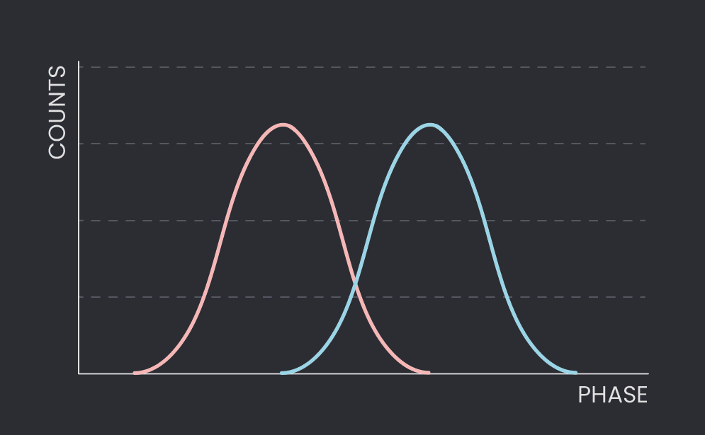
Measuring the state of a superconducting qubit involves measuring the phase of a signal reflected from its readout resonator. If we repeatedly send pulses and mature the phase upon reflection, we can draw a histogram, as seen in Figure 1. The counts eventually expose the state of the qubit, as seen by the two Gaussians in the figure – each resulting from a different qubit state (here ground in red, excited in blue).

That out of the way, our task is quite simple: make it such that the qubit is in the ground state. We measure the state of the qubit, and if it is already in the ground state, we don’t want to apply any gates, while if it’s in the excited state, we apply an X or a bit flip gate, to bring it to the ground state. Sounds simple enough, right?

In the simplest case, we can use a naive single-shot active reset approach. We define some threshold a. If the measurement outputs a phase greater than a, we apply a bit flip. This simple scheme can be seen in Figure 2. At first glance, this seems like a decent idea. However, we quickly encounter a problem. A tail of the excited qubit distribution exists left of the threshold a, meaning that it will not be caught and a bit flip won’t be applied (a false-negative result). Similarly, a ground state distribution tail falls to the right of the threshold a. Applying a bit flip to the ground state will do the opposite of what we want; it will bring the qubit to the excited state (a false-positive). As you may imagine, this poses a bit of a problem.

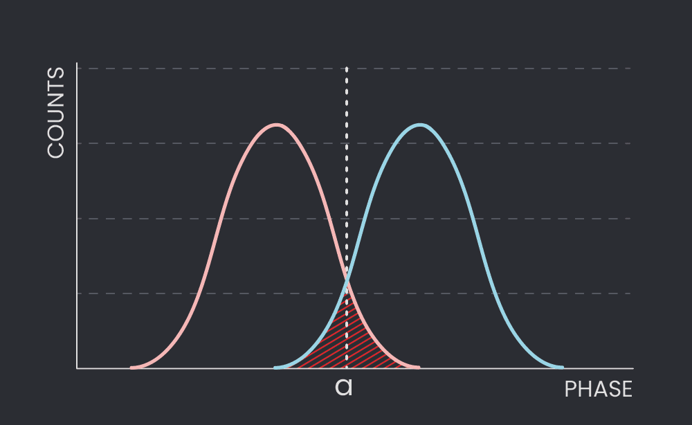
No matter how many times we repeat this operation, we will never be able to get a good enough initialization fidelity; it will be limited by the inherent measurement fidelity involved, which corresponds to the distance between the two peaks. The key here is that the only information we have access to is the phase; we do not know which distribution we sample from. Thus, we’re at a stalemate – we’ll be limited by measurement fidelity, which we can’t beat. 

Positive feedback – the light at the end of the tunnel

One solution comes in the form of a repeat-until-success active reset. We now add another threshold parameter that corresponds to the ground state peak’s frequency, which we dub p (see Figure 3). Having two thresholds changes the rules of the game: if we are to the left of p (and therefore a as well), we believe we’re firmly in the ground state regime, and we don’t do anything to our qubit. 

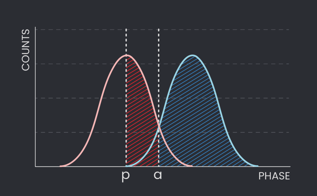
Now, what happens otherwise? If we measure to the right of a (blue region in Figure 3), we apply our bit flip, assuming that we were, in fact, in the excited state regime. If we’re between p and a (red region in Figure 3), we do nothing. The key here is that all of this happens in a while loop – after this, we measure our qubit once again. Sampling it once more allows us to glean some important information: we can see if we are now to the left of the peak p threshold – further validating we are in the ground state. If not, we once again follow the same protocol as above and look at the next iteration. We can keep sampling until the qubit is definitively sampled left of the peak p.

The pseudo-code is laughably simple and looks like this:

while (phase>p)
	if (phase>a)
	play (pi, qubit)

This provides an important change: our fidelity isn’t limited by the measurement fidelity – it is now limited by how much the excited state histogram penetrates past the g peak. Additionally, we can dynamically change the point p. We can push that threshold further to the left, giving us more peace of mind about measuring a qubit in the ground state – but of course, there’s always a trade-off;  the further you put the threshold to the left, the longer it will take you to be done with the reset protocol.

Another important takeaway is that this protocol is dynamic; it could take you 2 iterations or 10 to get your qubit in the ground state. In either case, the OPX+ evaluates if its work is done while it’s still doing the work – you don’t need to pre-program the iterations. In the case of an AWG, you’d need to load everything ahead of time – here, the FPGA is a ‘brain’ that is able to decide for itself when the conditions have been satisfied. This allows for a much more dynamic, interactive, and active way to work.

Active reset is a direct demonstration of the feedback capabilities afforded by QUA and the OPX+. It’s been successfully incorporated into experiments run by our customers from the very beginning of our journey at Quantum Machines. It runs to the core of what we do but is just the tip of the iceberg in terms of where feedback can get you. Ultimately it’s the same for physics researchers and their qubits: there’s no limit to where you can go with a bit of positive feedback, trying until you get it right and keeping active.