Finally, a Practical Way to Benchmark Quantum Controllers

The adoption of gate-level benchmarks such as Quantum Volume or CLOPS has offered an amazing way for researchers and industry leaders to compare and advance quantum computing technologies. These are metrics one can compare against, build roadmaps on, and overall use to track progress toward quantum advantage, both for NISQ applications and fault tolerance.

Although a lot of good came – and much is yet to come – thanks to gate-level metrics, these do not allow us to distinguish between the quality of qubits and the performance of the quantum controller. This makes it difficult to push the boundaries of each individually. If we really want to do our very best to achieve the fault-tolerant dream, we must be able to measure performance at all levels of the stack. This is why Quantum Machines was working to develop an additional framework for evaluating quantum control solutions specifically. A framework we are proud to share with you today.

Why Pulse-Level Benchmarks Matter

In our recent article (the pre-print is linked above), we propose a set of pulse-level benchmarks that allow measuring the performance of quantum controllers in a way that relates to practical applications and state-of-the-art quantum protocols. Pulse-level refers to the implementation of gates and the electromagnetic pulses in their making.

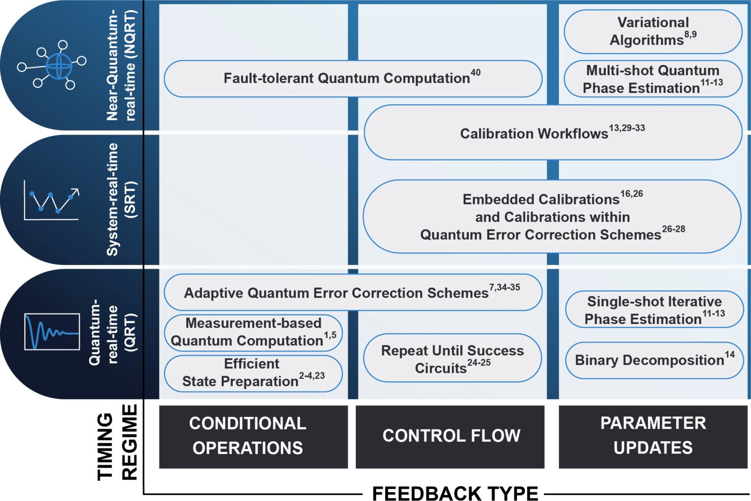
To properly understand the role of a quantum controller and how we can measure its performance, we divide the controller needed response time into three main timing regimes, called quantum-real-time (QRT), system-real-time (SRT), and near-real-time (NRT). These timeframes offer an understanding of what time we must compare to when evaluating a certain operation. For example, qubit rotations must happen faster than coherence time, QRT, while calibrations must happen faster than the drift of the parameter they aim at correcting, SRT.

Once the timing regime is clear, we discern between three main categories of feedback operation that need to be supported: conditional operations, full control flow, and parametric updates. These are the groups of operations that make the vast majority of the operations necessary for NISQ applications and are likely to bring the industry to fault tolerance. For example, most quantum protocols start with actively resetting the qubits. This is often done via a measurement followed by a conditional pi pulse. More complicated protocols require complicated branching with decision-making and control flow operations performed in real-time.

Within this framework, we categorize some of the most important protocols in the race toward quantum advantage, ensuring we measure what matters. In Figure 1 below, we show examples of required functionalities and use cases that the ideal quantum controller should support, divided into two conceptual dimensions: feedback types and timing regimes for such feedback to be useful.

Quantum Control Benchmarks for Active Reset

Let us dive into a specific example to understand what a quantum control benchmark looks like. We mentioned that at the beginning of most protocols, we would like to reset our quantum processing unit (QPU), i.e., our qubits. Resetting can be done actively, for example, by means of a strong single-shot measurement, followed by state discrimination and some more classical processing. This computation informs the decision of playing (or not) a conditional pi-pulse. Such protocol guarantees, with a high probability, to have our QPU in the ground state. Obviously, this is a simplified version of the much harder truth, which is that getting close to 100% fidelity is tough (there are ways to go about it that you can read about here). Generally, the decision-making might be local, i.e., relating to information from a single controller channel, or aggregated, i.e., taking in information from multiple channels. Still, its duration is one of the components of the time necessary to perform the operation.

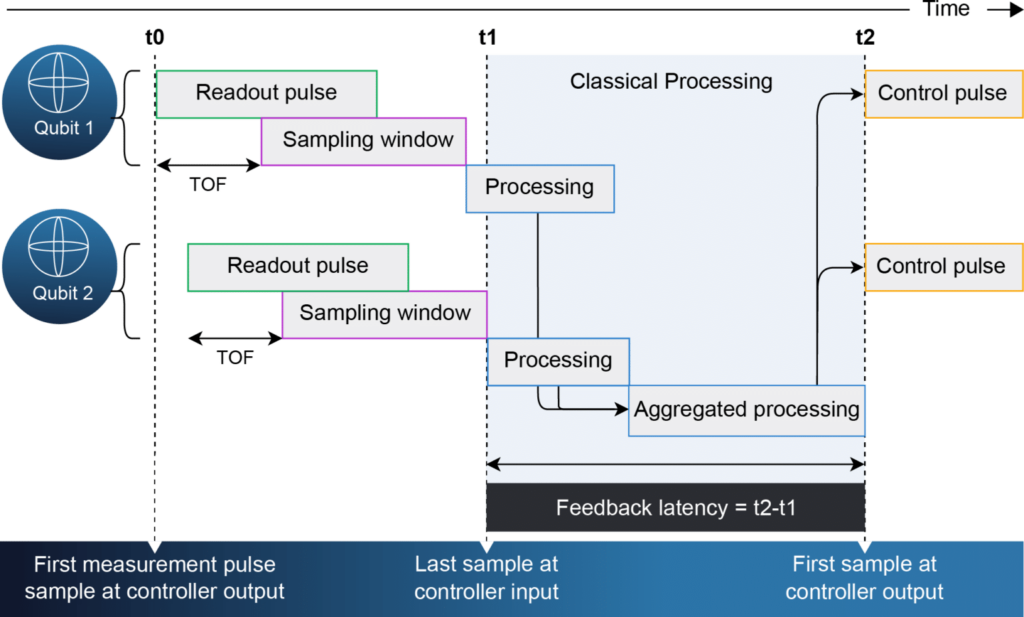
In Figure 2 below, we show the Timeline of controller operations for a generalized feedback sequence. The controller feedback latency is defined as the time from the last sample required for the calculation that affects the output is sampled (t1) until the first sample of the dependent pulses is sent at the controller output (t2).

Measuring Feedback Latency

Within this important procedure and much like the control pulse, the parameters of the readout pulse and sampling window mostly depend on the qubits, which have to be carefully calibrated. It should be clear that we would like our controller to minimize the feedback latency, the time between the last sampling point and the first reaction. If this delay was zero, we would be very happy, as the whole operation would be limited by the physical system we are trying to control rather than our controller.

In reality, analyzing data and performing any processing takes a non-negligible amount of time. For example, the OPX+ performs an active reset with a latency of about 200ns. Now to put this into perspective and understand whether it is good or bad, we need to know more about the actual implementation and the qubits. What we know is that this time must be compared with the coherence time of the QPU. Is 200ns much lower than your qubit’s lifetime? Is controller latency the bottleneck in your quantum operations?

To measure the feedback latency, one way is to utilize the controller’s knowledge about the timing of the pulses sent to the qubit. In the code below, we utilize our quantum universal assembly (QUA), the first pulse-level programming language, to define this implementation. If we call the time of the first sample of the readout pulse re_time, and the time of the first sample of the control pulse ce_time, we have a straightforward way to calculate the latency by subtracting from this delay the time of flight and the sampling window size, which are both calibrated measurements.

def benchmark_deterministic_QRT_conditinal_operation():
   fixed x
   bool s

   strict_timing:
      measure(readout_pulse, readout_element, demod(x), timestamp-> re_time)
      s = x > 0
      wait(max_time=max_latency, control_element)
      play(control_pulse, control_element, condition = s, timestamp-> ce_time)

   return feedback_latency = ce_time - (re_time + sampling_window + time_of_flight)

Code 1: QUA code defining the BM1.1 benchmark for QRT conditional operations. Green: elements of the configuration file. Blue: real-time classical variables. Red: pulse-level commands. Orange: constants. 

This is a simple measurement that any control instrument should be able to support and that evaluates a metric of practical interest for the vast majority of quantum protocols. It is very hard to imagine NISQ applications and quantum advantage happening without such an active reset protocol involved. This is especially true when considering large, many-qubits QPUs.

And this is Just the Beginning

This blog gives you a taste of what real, practical quantum control benchmarks are like. Our work covers a multitude of important requirements and use cases and offers similar codes to implement practical tests on any quantum controller. This becomes much more interesting and more complex when discussing complicated branching, calibrations embedded within quantum circuits, or operations involving multiple qubits and measurements spread in time. We invite you to take a deeper dive into quantum control benchmarking and to have a look at the pre-print below!

Yours,
Lorenzo